1 INTRODUCTION
Material consumption, as a critical component of the overall construction cost and carbon emissions, has been widely concerned in the design of building structures (Elfaki et al., 2014; Gan et al., 2020; Sharma et al., 2021). Contractors typically consider construction material quantity (CMQ) as an important aspect in selecting a structural design scheme that can achieve the minimum estimated overall construction cost. Furthermore, CMQ is directly related to the carbon emissions of the construction industry, which must be reduced to realize carbon neutrality and achieve the United Nations Sustainability Development Goals (SDGs) (UNEP, 2022). Although CMQ only affects a portion of the building budget and lifetime carbon footprint, it is the primary component that can be optimized through structural design. Hence, the design objectives of computer-aided structural design methods typically include CMQ minimization (Afzal et al., 2020; M¨˘laga-Chuquitaype, 2022).
Reinforced concrete (RC) buildings are among the most widely used structural types being built with concrete and reinforcing steel. Steel consumption, which is relatively difficult to estimate, is a major concern for engineers in practical projects due to its significant impact on the construction cost. Concrete consumption is also gaining increasing attention nowadays after the SDGs become an urgent call for action by all countries. Currently, the mainstream CMQ estimation methods for RC buildings can be classified into three categories.
Category 1: Simplified formulas can be used to estimate CMQ (Sharafi et al., 2012; Zhang & Mueller, 2017; Zhou et al., 2022). In this category, the methods are highly efficient; however, they typically either display low accuracy or are only applicable to simple structural systems, such as frame structures.
Category 2: Structural design software, which is used to conduct detailed design, can also estimate the corresponding concrete and steel consumptions (Kim et al., 2013; El-Sokkary & Galal, 2020; Zhang et al., 2021). This method is the most accurate; however, it highly relies on a complicated physics-based analysis model and is therefore time-consuming and inefficient, normally requiring 1¨C10 minutes of calculation time for a typical RC building. Among computer-aided optimization design techniques, heuristic methods are usually recognized as effective and practical (Aldwaik & Adeli, 2014). The possibility of finding the optimal solution by heuristic methods is positively related to the number of evaluated solutions in the design space. Typically, heuristic methods require hundreds of evaluations during iterations before finding a rational solution (Adeli & Sarma, 2006; Boscardin et al., 2019; Zhang et al., 2023). Another kind of emerging design technique is artificial intelligence (AI)-based methods (M¨˘laga-Chuquitaype, 2022). During the training of AI models, the prediction results must be evaluated to guide parameter updating. Due to the nature of big data, at least thousands of evaluations are needed for training. Consequently, with the current level of efficiency of structural design software in obtaining the CMQs of RC buildings, design and optimization requirements are difficult to meet. To reduce the computational cost, surrogate models have been proposed, as discussed in the next category.
Category 3: The CMQ can be estimated using AI-based or data-driven methods (Idowu & Lam, 2020; Antoniou et al., 2023; Kovačević et al., 2023), which allows a good balance to be achieved between accuracy and efficiency. They have been widely used as surrogate models to evaluate the objective functions of evolutionary algorithms (Jin et al., 2019; Chugh et al., 2019). The foregoing is the focus of this study as elaborated in the following sections.
The fundamental paradigm of data-driven CMQ estimation methods lies in three aspects (Singh, 1991; Yeh, 1998; Son et al., 2013; Fragkakis et al., 2015; Garc¨Şa de Soto et al., 2014; Dimitriou et al., 2018; Beljkaš et al., 2020; Idowu & Lam, 2020; Kovačević et al., 2023; Antoniou et al., 2023). (1) Real-world engineering cases are collected, and CMQs are used as label data. (2) Key features are manually selected as input data. (3) A data-driven model is selected to establish the mapping relationship between inputs and labels. However, the existing research on this paradigm has the following limitations: (a) The number of engineering cases collected is typically limited; therefore, the generalization of the model requires further exploration. (b) CMQ is affected by heterogeneous data such as component layout (topology), component section size (geometry), and design conditions (text). However, due to the limitations of their model architecture, existing methods cannot directly handle this data and require manual feature selection, which is inevitably restricted by the knowledge and experience of the developers. (c) A data-driven model is a ˇ°black boxˇ±, which is not guided by prior knowledge; consequently, it is prone to fundamental errors.
In recent years, intelligent structural design methods based on generative AI have developed rapidly (Liao et al., 2021; Fu et al., 2023). This technology can quickly generate numerous structural designs and provide valuable data that can be applied to real-world engineering cases. Deep learning models can automatically mine high-dimensional hidden features from data, thereby avoiding the subjectivity of manually defined input features. In addition, in previous research, the authors have successfully integrated engineering knowledge into deep learning, effectively improving the reliability of data-driven models (Fei et al., 2022a; Lu et al., 2022). These previous studies have established a solid foundation for the present study.
Specifically, this study proposes to establish the following strategies to solve the problems that have been encountered by the existing studies. (1) A data augmentation method is proposed, incorporating generative adversarial networks (GANs) and parametric modeling. A considerable amount of synthetic data is generated, and therefore dataset diversity is enriched. (2) A graph neural network (GNN) architecture is proposed herein, which enables direct mapping from all related information to CMQs through a heterogeneous feature fusion mechanism, thereby curtailing the limitations of manually selected features. (3) A prior knowledge inclusion strategy is proposed, which avoids fundamental errors by modifying the output layer and the loss function of the GNNs.
To validate the effectiveness of the proposed methods, RC shear wall building structures, typically used in high-rise residential buildings, are considered as practical examples. The CMQs of these buildings are difficult to estimate because of the presence of shear walls, but are a key factor that must be considered in structural design. Accordingly, the use of a data-driven method to accurately and efficiently estimate the CMQs of RC shear wall building structures is desirable.
The remainder of this paper is organized as follows. Section 2 reviews related studies. Section 3 presents the outline of a novel CMQ estimation method for RC buildings. Section 4 introduces the knowledge-enhanced GNN specifically designed for CMQ estimations. Section 5 describes the data augmentation of the CMQ dataset based on GANs and parametric modeling. Section 6 introduces three other data-driven methods for comparison. Section 7 presents the numerical experiments. Section 8 discusses the case study of several shear wall structures of residential buildings. Finally, the conclusions of this study are presented in Section 9.
2 REVIEW OF CURRENT LITERATURE
2.1 Data-driven CMQ estimation
The research on CMQ estimation using data-driven methods can be traced back to the 1990s (Singh, 1991), and continues to advance recently (Antoniou et al., 2023). The common methods used in relevant research include artificial neural network (ANN) (Adeli & Wu, 1998; Dimitriou et al., 2018; Beljkaš et al., 2020), support vector machine (Idowu & Lam, 2020), and regression analysis (Fragkakis et al., 2015; Son et al., 2013). The research targets include buildings (Garc¨Şa de Soto et al., 2014; Idowu & Lam, 2020), bridges (Beljkaš et al., 2020; Kovačević et al., 2023), and civil infrastructures (Fragkakis et al., 2015; Antoniou et al., 2023).
Similarly, a significant amount of research is dedicated to estimating construction costs (Adeli & Wu, 1998; Rafiei & Adeli, 2018). These estimation methods are widely used in the cost optimization of concrete structures (Ahmadkhanlou & Adeli, 2005; Aldwaik & Adeli, 2016), steel structures (Sarma & Adeli, 2000a; Sarma & Adeli, 2000b), and composite structures (Kim & Adeli, 2001; Adeli & Kim, 2001). This study mainly focuses on the CMQ estimation because the material cost can be easily calculated based on CMQ if the material price is provided.
Table 1 summarizes some related studies on CMQ estimation of RC structures, including the target, method, number of variables, data size, and prediction error measured by the mean absolute percentage error (MAPE) (if applicable). These studies support the decision-making of stakeholders of construction projects by estimating CMQs. These estimations can be used in design optimization as long as the design variables of RC structures are included as the input variables of the data-driven model. The ground truth of the CMQs is obtained from the design documents, especially the bill of quantities. The accuracy of existing methods (2% ˇÜ MAPE ˇÜ 30%) is influenced by many factors and is in need of further improvement. These factors include: (1) only a small number of manually selected variables (three to ten) are considered and the methods may have overlooked useful information that developers are not aware of; (2) data-driven models are prone to fundamental errors if no prior knowledge is incorporated; (3) the data size (or the number of different RC structure samples) is small (6 to 400) compared to those of nowadaysˇŻ big data tasks (Sun et al., 2017), and the sample diversity is limited. The above-mentioned factors are further discussed in Sections 2.2, 2.3, and 2.4, respectively.
TABLE 1. Related studies on CMQ estimation of RC structures
|
Reference |
Target |
Method |
Number of variables |
Data size |
Concrete MAPE (%) |
Steel MAPE (%) |
|
Antoniou et al., 2023 |
Metro station |
RA/ANN |
5 |
6 |
2.13 |
14.77 |
|
Kovacevic et al., 2023 |
Bridge |
GPR |
6 |
181 |
11.65 |
N/A |
|
Idowu & Lam, 2020 |
Building |
SVM |
10 |
80 |
12.19~28.35 |
12.59~29.73 |
|
Beljkas et al., 2020 |
Bridge |
ANN |
6 |
101 |
8.56 |
17.31 |
|
Dimitriou et al., 2017 |
Bridge |
ANN |
5 |
68 |
37 |
31 |
|
Garc¨Şa de Soto et al., 2015 |
Building |
RA/ANN |
7 |
58 |
3.48 |
7.44 |
|
Fragkakis et al., 2015 |
Culvert |
RA |
3 |
104 |
13.78 |
19.79 |
|
Yeh, 1998 |
Building |
ANN |
10 |
400 |
N/A |
5.5~14.7 |
Note: RA=Regression Analysis; ANN=Artificial Neural Networks; GPR=Gaussian Process Regression; SVM=Support Vector Machine; MAPE=Mean Absolute Percentage Error; N/A=Not Applicable.
2.2 Graph neural networks
With the development of deep learning technology, deep neural networks can automatically extract key features from massive amounts of information. Deep learning approaches are gradually replacing traditional feature engineering methods in the fields of computer vision and natural language processing (Russakovsky et al., 2015; Bubeck et al., 2023).
GNN is a type of deep learning approach that operates on graphs, a data structure that represents a set of objects (nodes) and their relationships (edges) (Zhou et al., 2020). In recent years, variants of GNNs such as graph convolutional networks (GCN) (Kipf & Welling, 2016) and Graph-SAGE (Hamilton et al., 2018) have exhibited excellent performances on many deep learning tasks. Nowadays, the applications of GNN have been extended to various tasks with graph-like data structures, such as building structures (Song et al., 2022; Zhao et al., 2023a), water distribution networks (Fan et al., 2023), package-based constraint management (Wu et al., 2023), autonomous vehicle networks (Chen et al., 2021), neural network architectures (Xue et al., 2021), neural signals (Feng et al., 2021), and electroencephalogram signals (Zhao et al., 2021; Che et al., 2022; Lian & Xu, 2022).
However, existing GNNs cannot be directly applied to CMQ estimation because of the heterogeneous input data of this task, including component layout (topology), component section sizes (geometry), and design conditions (text). Hence, this study proposes a novel GNN architecture with a heterogeneous feature fusion mechanism, so that all related information can be directly input into the model without specifying any features artificially.
2.3 Knowledge-enhanced neural networks
Two principal rules must be satisfied to achieve the CMQ estimation of RC buildings based on prior knowledge in structural engineering practice. (1) The total concrete consumption of a building structure is less than the sum of the calculated volumes of all structural components. This is due to the common duplications in calculating the volumes of components. For example, doubling the concrete volume of overlapped beam¨Ccolumn joints must be avoided. (2) The amount of steel reinforcement for any structural component must satisfy the minimum requirements specified in the design codes (MOHURD, 2010, 2015, 2016). However, to the best knowledge of the authors, such prior knowledge has not been considered in the existing data-driven CMQ estimation methods. Hence, unexpected major and fundamental errors may occur during the data-driven model estimation process considering the statistical nature of such models.
Generally, for neural networks, prior knowledge is introduced by modifying the following three elements of the network (Dash et al., 2022): (1) input data (Yin et al., 2019; Marino et al., 2021), (2) loss function (Lu et al., 2022; Fei et al., 2022a; Du et al., 2022), and (3) network architecture (Sourek et al., 2018; Du et al., 2020; Li et al., 2021). The second element, viz., modifying the loss function, is adopted in this study. The output layer of the neural networks is also modified to ensure 100% satisfaction of the prior knowledge.
2.4 Data augmentation of structural design
Table 1 indicates that the data sizes used in the existing studies are no larger than 400, which is much smaller than those of typical deep learning tasks (Sun et al., 2017). This may result in a limited generalization of trained models and difficulty in applying them to practical projects. Since collecting large-scale real-world engineering project data is costly or even unattainable under certain circumstances (DˇŻAmico et al., 2019), the use of synthetic data generated by generative AI to supplement real-world data is desirable.
Structural design methods based on AI have emerged rapidly in recent years and have received extensive attention (Adeli, 2020; Sun et al., 2021; M¨˘laga-Chuquitaype, 2022). The AI technologies used in relevant research projects include GANs (Zhang et al., 2021; Khan et al., 2023), GNNs (Wang & Zhang, 2021; Chang & Cheng, 2020), convolutional neural networks (CNNs) (Yu et al., 2019; Ampanavos et al., 2022), and reinforcement learning (Hayashi & Ohsaki, 2021; Jeong & Jo, 2021). In particular, a series of research studies have focused on GAN-based design methods for building structures, providing a good foundation for this study (Pizarro et al., 2021; Liao et al., 2021; Fu et al., 2023).
The GAN approach is also a well-recognized data augmentation method (Shorten & Khoshgoftaar, 2019) that can generate realistic synthetic data. However, it has yet to be applied to CMQ estimation tasks because of the difficulty in automatically obtaining the CMQ of synthetic structural design. Therefore, this study proposes a data augmentation method, combining parametric modeling with the GAN-based design method, thereby increasing the CMQ data size by an order of magnitude.
3 Outline of the proposed CMQ estimation method
This study aims to resolve the problems encountered in the CMQ estimation of RC buildings. Consider an RC shear wall building structure as an example. Given the actual structural design (including the spatial layout and geometric dimensions of shear walls and beams) and design conditions (including seismic, site, and height conditions), the concrete and steel consumptions (of shear walls, beams, and slabs) are estimated. The CMQ estimation method proposed in this study, including three modules, is shown in Figure 1.
(1) Model application module: The structural design and design conditions to be considered are represented as a graph (Section 4.1). The concrete and steel consumptions are estimated by inputting the graph into a trained GNN model (Section 4.2). The GNN parameters are generated from Module (2).
(2) Model training module: The GNN model is trained based on the CMQ dataset. The model can extract and fuse Global, Edge, and Node features, and is thereby named as Graph-GEN. It can also embed prior knowledge to ensure that the CMQ estimation satisfies the principal rules of not exceeding the maximum concrete consumption and not below the minimum steel consumption (Section 4.3). The CMQ dataset, including input and label data, is generated from Module (3).
(3) Data augmentation module: A GAN model is trained using a dataset collected from real-world engineering projects. It is then used to generate a large number of synthetic structural designs corresponding to synthetic design conditions. After that, refined finite element models are established using parametric modeling, and their CMQs are determined. This process expands the size of the CMQ dataset by an order of magnitude, thus facilitating the effective training of Graph-GEN (Section 5).
4 Knowledge-enhanced GNNs
A novel GNN architecture called Graph-GEN is proposed that incorporates a heterogeneous feature fusion mechanism and a prior knowledge inclusion strategy. It is capable of extracting and fusing high-dimensional features in various forms, including component layout (topology), component section sizes (geometry), and design conditions (text), which are subsequently mapped into CMQs. Innovatively, prior knowledge is introduced into Graph-GEN by modifying the loss function and output layer.
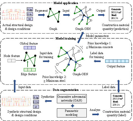
Figure 1. The proposed CMQ estimation method
4.1 Feature representation ¨C model application module
To use a GNN for CMQ estimation, the structural design of an RC building must be represented as a graph. A straightforward approach is adopted to represent the topological relationship of structural components. It is applicable to walls, columns, beams, braces, and so forth, where the structural components are represented by graph edges and the intersections of the structural components are represented by graph nodes (Zhao et al., 2023b). Among all the floors of a building structure, a standard floor can best represent the planar layout of structural components. Therefore, a standard floor of a shear wall building structure is considered herein as an example. The planar layout of the shear walls and beams is represented as a graph, as shown in Figure 2, in which the coordinates of the intersections are used as node features, and the geometric dimensions of the structural components are used as edge features. Thus, all the structural design information can be represented as a graph. For this standard floor of a shear wall building structure, the node features are two-dimensional vectors containing the X and Y coordinates, and the edge features are three-dimensional vectors comprising the length, width, and height of the structural components, as described in Table 2.
Design conditions also
significantly affect the CMQ estimation of a building structure (MOHURD, 2010).
For example, if a building structure is subjected to a large horizontal seismic
action, the amount of reinforcement of the vertical components on the ground
floor must increase accordingly. For shear wall building structures, three design
conditions are selected for illustration, including seismic, site, and height
design conditions, which are represented by the design seismic acceleration
( ![]() ), the site characteristic period (
), the site characteristic period ( ![]() ), and the number of floors (
), and the number of floors ( ![]() ), respectively (MOHURD, 2016). Further details are provided in Appendix
A. The foregoing design conditions are also represented as a three-dimensional
vector known as a global feature because they affect the CMQs of all structural
components, as shown in Table 2. The global feature is highly scalable, and
its size can be adjusted to consider various design conditions.
), respectively (MOHURD, 2016). Further details are provided in Appendix
A. The foregoing design conditions are also represented as a three-dimensional
vector known as a global feature because they affect the CMQs of all structural
components, as shown in Table 2. The global feature is highly scalable, and
its size can be adjusted to consider various design conditions.
The CMQs to be predicted are represented as six-dimensional or two-dimensional vectors comprising the concrete and steel consumptions of shear walls, beams, and slabs (separated or combined), as given in Table 2. These two representations will be discussed in Section 7.2.
TABLE 2. Input and output variables of Graph-GEN
|
Variable |
Representation form |
|
|
Input |
Graph |
Node set
|
|
Node features {
|
|
|
|
Edge features {
|
|
|
|
Global features
|
|
|
|
Output |
Vector representations
|
|
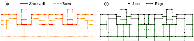
FIGURE 2. Graph representation of shear wall building structure: (a) planar layout of shear walls and beams; (b) graph nodes and edges
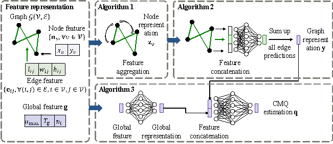
Figure 3. Graph-GEN architecture
4.2 Model architecture - Graph-GEN
Given the fact that both the structural design (represented by a graph) and design conditions (represented by a vector) significantly affect the CMQs, this study therefore proposes a novel GNN architecture, named Graph-GEN, which extracts and fuses Global, Edge, and Node features, as demostrated in Figure 3.
Firstly, each node representation is generated by aggregating the representations of its adjacent nodes and the features of its incident edges, the intuitive meaning of which is the CMQ requirements of structural joints (Algorithm 1 in Figure 3). Secondly, each edge prediction is generated using the representations of itself and its end nodes, with an intuitive meaning being the CMQ in each structural component. All edge predictions are then summed up into a graph representation, intuitively standing for an initial CMQ estimation (Algorithm 2 in Figure 3). Thirdly, the processed global features (design conditions) and the graph representation are concatenated and mapped into the final CMQ estimation (Algorithm 3 in Figure 3). The core algorithms with matching steps are introduced below, and the input and output features have been described in Section 4.1.
Step 1: Input the graph
![]() , node features
, node features ![]() , and edge features
, and edge features ![]() into the GNN layers to generate the node representations
into the GNN layers to generate the node representations
![]() . The GNN layer is constructed upon Graph-SAGE (Hamilton et al., 2018)
and improved to consider the edge features (geometric dimensions of the structural
components) (Zhao et al., 2023a).
. The GNN layer is constructed upon Graph-SAGE (Hamilton et al., 2018)
and improved to consider the edge features (geometric dimensions of the structural
components) (Zhao et al., 2023a).
Algorithm 1 describes
the feature aggregation process of Graph-GEN (Figure 3). For the k-th
GNN layer, each node first concatenates the current node representations
![]() , the edge features
, the edge features ![]() , and the neighbor node representations
, and the neighbor node representations ![]() . Then, the concatenated vector is fed into a fully connected layer
with non-linear activation and mapped into a temporary vector. After that, all
temporary vectors in the immediate neighborhood are summed up into a single
vector
. Then, the concatenated vector is fed into a fully connected layer
with non-linear activation and mapped into a temporary vector. After that, all
temporary vectors in the immediate neighborhood are summed up into a single
vector ![]() . This vector is concatenated with the nodeˇŻs current representation
. This vector is concatenated with the nodeˇŻs current representation
![]() . Note that for the first GNN layer, the node representation
. Note that for the first GNN layer, the node representation
![]() is the input node feature. The concatenated vector is again
fed into a fully connected layer with non-linear activation and mapped into
an updated node representation
is the input node feature. The concatenated vector is again
fed into a fully connected layer with non-linear activation and mapped into
an updated node representation ![]() to be used in the next GNN layer.
to be used in the next GNN layer.
Algorithm 1. Feature aggregation of Graph-GEN
|
Input: |
Graph |
|
Output: |
Vector representation |
|
for for end for end for |
|
Step 2: Based on the updated
node representations ![]() and non-updated edge features
and non-updated edge features ![]() , the edge predictions and the graph representation
, the edge predictions and the graph representation ![]() can be obtained (Figure 3). Specifically, this is accomplished
by concatenating the edge feature and end node representations of each edge,
and passing the concatenated vector to fully connected layers with non-linear
activation to obtain the edge prediction (Zhao et al., 2023a). Since this
operation is performed on the edge level, the size of the weight matrices is
irrelevant to the size of the input graph. Subsequently, all edge predictions
are summed into one vector and passed onto the fully connected layers with non-linear
activation to obtain the graph representation y. Summing all edge predictions
ensures that the size of the graph representation y is consistent and
irrelevant to the size of the input graph. This approach is intuitive. First,
the CMQs of each structural component are estimated by simultaneously considering
the structural component itself (edge feature) and the joints at both of its
ends (end node representations). Then, the preliminary CMQs of the entire building
structure are obtained by summing those of all structural components. Algorithm
2 below provides further details. Note that Algorithm 2 is different from the
existing methods in its unique way to obtain the graph representation, considering
all edge and node features.
can be obtained (Figure 3). Specifically, this is accomplished
by concatenating the edge feature and end node representations of each edge,
and passing the concatenated vector to fully connected layers with non-linear
activation to obtain the edge prediction (Zhao et al., 2023a). Since this
operation is performed on the edge level, the size of the weight matrices is
irrelevant to the size of the input graph. Subsequently, all edge predictions
are summed into one vector and passed onto the fully connected layers with non-linear
activation to obtain the graph representation y. Summing all edge predictions
ensures that the size of the graph representation y is consistent and
irrelevant to the size of the input graph. This approach is intuitive. First,
the CMQs of each structural component are estimated by simultaneously considering
the structural component itself (edge feature) and the joints at both of its
ends (end node representations). Then, the preliminary CMQs of the entire building
structure are obtained by summing those of all structural components. Algorithm
2 below provides further details. Note that Algorithm 2 is different from the
existing methods in its unique way to obtain the graph representation, considering
all edge and node features.
Algorithm 2. Global representation of Graph-GEN
|
Input: |
Graph |
|
Output: |
Vector representation |
|
for for end for end for |
|
Step 3: The CMQs can be
estimated based on the graph representation ![]() and the global feature
and the global feature ![]() . Specifically, the global feature is inputted into the fully connected
layers with non-linear activation, and the output vector is concatenated with
the graph representation. The concatenated vector is then inputted into the
fully connected layers with non-linear activation and mapped as the CMQ representation
. Specifically, the global feature is inputted into the fully connected
layers with non-linear activation, and the output vector is concatenated with
the graph representation. The concatenated vector is then inputted into the
fully connected layers with non-linear activation and mapped as the CMQ representation
![]() (Figure 3). The intuitive attribute of this
approach is to use the global features (design conditions) to adjust the graph
representations (preliminary CMQs). Further details are provided in Algorithm
3 below. Note that the novelty of Algorithm 3 lies in its separate processing
of the global feature and effective fusion of heterogeneous features.
(Figure 3). The intuitive attribute of this
approach is to use the global features (design conditions) to adjust the graph
representations (preliminary CMQs). Further details are provided in Algorithm
3 below. Note that the novelty of Algorithm 3 lies in its separate processing
of the global feature and effective fusion of heterogeneous features.
Details of Graph-GEN architecture, including the specific setting of each neural network layer, can be found in Appendix B. Three architecture settings are presented with different graph depth K, fully connected layer depths M and N, and are later discussed in Section 7.1.
Algorithm 3. Feature fusion of Graph-GEN
|
Input: |
Graph representation |
|
Output: |
Vector representation |
|
for |
|
|
end for |
|
4.3 Knowledge inclusion - model training module
In the CMQ estimation task for RC buildings, the following prior knowledge described in Section 2.3 is elaborated herein.
(1) The total concrete consumption of the building structure is less than the sum of the calculated volumes of all structural components. This is apparent because an inevitable duplication exists in calculating the volumes of structural components. The concrete volume of the overlapped regions (e.g., beam¨Ccolumn and beam¨Cwall joints) must not be doubly counted.
(2) The steel consumption of any structural component must satisfy the minimum reinforcement requirements as specified in the design codes (MOHURD, 2010, 2015, 2016). Evidently, this prior knowledge must be determined according to the local codes. For the RC shear wall building structures constructed in China, the minimum reinforcement requirements for shear walls, beams, and slabs are presented in Appendix C.
This study introduces
the foregoing prior knowledge into data-driven models by modifying the loss
function and output layer. Specifically, to ensure that the prior knowledge
is 100% satisfied, knowledge transformations are performed at the output layer,
and a knowledge inclusion loss function ( ![]() ) is derived based on these transformations (Dash et al., 2022). This
approach is applicable not only to the proposed Graph-GEN but also to other
neural network-based models. The loss function of such knowledge-enhanced neural
networks is expressed by Equations (1)¨C(3):
) is derived based on these transformations (Dash et al., 2022). This
approach is applicable not only to the proposed Graph-GEN but also to other
neural network-based models. The loss function of such knowledge-enhanced neural
networks is expressed by Equations (1)¨C(3):
|
|
(1) |
|
|
|
(2) |
|
|
|
(3) |
where ![]() is the loss function of knowledge-enhanced neural networks;
is the loss function of knowledge-enhanced neural networks;
![]() is the data-driven loss function;
is the data-driven loss function; ![]() is the knowledge inclusion loss function;
is the knowledge inclusion loss function; ![]() is the mean square error loss function;
is the mean square error loss function; ![]() returns the zero tensor of the same shape as the input tensor;
and
returns the zero tensor of the same shape as the input tensor;
and ![]() is the weight of knowledge loss (
is the weight of knowledge loss ( ![]() );
); ![]() and
and ![]() are the labels of concrete and steel consumptions, respectively.
are the labels of concrete and steel consumptions, respectively.
![]() and
and ![]() are the concrete and steel consumptions after the transformations,
as given by Equations (4) and (5), respectively.
are the concrete and steel consumptions after the transformations,
as given by Equations (4) and (5), respectively.
|
|
(4) |
|
|
|
(5) |
where ![]() is the weight of knowledge transformation (
is the weight of knowledge transformation ( ![]() );
); ![]() and
and ![]() are the concrete and steel consumptions directly outputted
by the neural networks, respectively;
are the concrete and steel consumptions directly outputted
by the neural networks, respectively; ![]() and
and ![]() are the portions of concrete and steel consumptions that
do not conform to the prior knowledge, as given by Equations (6) and (7), respectively.
are the portions of concrete and steel consumptions that
do not conform to the prior knowledge, as given by Equations (6) and (7), respectively.
|
|
(6) |
|
|
|
(7) |
where ![]() is the rectified linear unit activation function;
is the rectified linear unit activation function; ![]() and
and ![]() are the adjusting factors obtained from datasets, as given
by Equations (8) and (9).
are the adjusting factors obtained from datasets, as given
by Equations (8) and (9).
|
|
(8) |
|
|
|
(9) |
where ![]() and
and ![]() are the labels for concrete and steel consumptions of the
i-th sample, respectively;
are the labels for concrete and steel consumptions of the
i-th sample, respectively; ![]() and
and ![]() are the maximum concrete and minimum steel consumptions of
the i-th sample, respectively; N is the number of samples in the
dataset; Min{ˇ¤} and Max{ˇ¤} return the minimum and maximum elements in the list,
respectively.
are the maximum concrete and minimum steel consumptions of
the i-th sample, respectively; N is the number of samples in the
dataset; Min{ˇ¤} and Max{ˇ¤} return the minimum and maximum elements in the list,
respectively.
![]() and
and ![]() are the maximum concrete and minimum steel consumptions calculated
according to prior knowledge, as given by Equations (10) and (11) (for RC shear
wall building structures), respectively.
are the maximum concrete and minimum steel consumptions calculated
according to prior knowledge, as given by Equations (10) and (11) (for RC shear
wall building structures), respectively.
|
|
(10) |
|
|
|
(11) |
where ![]() ,
, ![]() , and
, and ![]() are the calculated volumes of a single shear wall, beam,
and slab, respectively (the steel volume is neglected);
are the calculated volumes of a single shear wall, beam,
and slab, respectively (the steel volume is neglected); ![]() ,
, ![]() , and
, and ![]() are the minimum steel consumptions of a single shear wall,
beam, and slab, respectively, calculated according to the minimum reinforcement
requirements given in Appendix C.
are the minimum steel consumptions of a single shear wall,
beam, and slab, respectively, calculated according to the minimum reinforcement
requirements given in Appendix C.
Note that the values of
![]() and
and ![]() have significant impacts on the model performance, especially
in extreme cases when
have significant impacts on the model performance, especially
in extreme cases when ![]() or
or ![]() ; this is discussed in Section 7.3.
; this is discussed in Section 7.3.
5 Data augmentation module
The performance and generalization of data-driven models are closely related to their data size. As mentioned in Section 2.1, collecting a number of real-world engineering design cases much larger than 400 for CMQ estimation is rather challenging. Therefore, this study proposes a data augmentation method based on GAN and parametric modeling to expand the size of the CMQ dataset by an order of magnitude. First, the GAN is trained based on real-world design data. Subsequently, a large amount of synthetic design data is generated using GAN. Finally, the CMQs corresponding to the synthetic design data are obtained using parametric modeling. To provide a specific explanation of the foregoing, consider an RC shear wall building structure again as an example.
5.1 Structural design dataset
To train the GAN, a structural design dataset containing 430 input data-output data pairs is collected from real-world engineering projects involving shear wall structures of residential buildings, as illustrated in Figure 4. Note that the data size (430) will be increased following data augmentation.
Each data pair includes
input and label data. The input data refer to the architectural design (planar
layout of partition walls, doors, and windows) and design conditions (
![]() ,
, ![]() , and
, and ![]() , as described in Section 4.1). The label data denote the structural
design (planar layout of shear walls, which is critical in the schematic design
of shear wall building structures). The architectural and structural designs
are represented as pixel images, and the design conditions are represented as
text (Liao et al., 2022). The real-world dataset is split into two parts: 80%
of the dataset is used for training and validation, and 20% is set aside for
testing.
, as described in Section 4.1). The label data denote the structural
design (planar layout of shear walls, which is critical in the schematic design
of shear wall building structures). The architectural and structural designs
are represented as pixel images, and the design conditions are represented as
text (Liao et al., 2022). The real-world dataset is split into two parts: 80%
of the dataset is used for training and validation, and 20% is set aside for
testing.
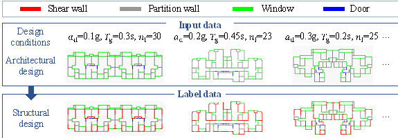
Figure 4. Structural design dataset
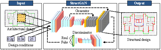
Figure 5. StructGAN architecture
5.2 StructGAN
A well-established GAN model, called StructGAN (Liao et al., 2022), is adopted in this study, as shown in Figure 5. StructGAN consists of a generator and a discriminator, both being deep neural networks. Through a zero-sum game between the generator and discriminator, StructGAN is able to reproduce the probability distribution of the label data based on the input data, thereby establishing a mapping relationship between the input and output. StructGAN is specially proposed for shear wall structure design. Its input is the architectural design being represented by a pixel image and design conditions being represented by texts. Its output is the structural design also being represented by a pixel image. For a given input architectural design, StructGAN can generate different structural designs in response to changes in design conditions.
StructGAN is trained on
the structural design dataset described in Section 5.1 (only the training set
is used, which is 80% of the 430 data pairs). After training, StructGAN is used
to generate synthetic structural designs. For each actual architectural design
as input, 10 synthetic design condition combinations are randomly selected.
The possible values of ![]() ,
, ![]() , and
, and ![]() are as follows:
are as follows: ![]() ,
, ![]() , and
, and ![]() . By doing so, 10 synthetic structural designs are obtained by StructGAN
for each actual architectural design. In consequence, the size of the structural
design dataset is increased by 10 times.
. By doing so, 10 synthetic structural designs are obtained by StructGAN
for each actual architectural design. In consequence, the size of the structural
design dataset is increased by 10 times.
Note that synthetic structural designs are automatically converted from pixel images into vector data using computer vision techniques previously proposed by our team (Fei et al., 2022b).
5.3 Parametric modeling
As described in Section 5.2, the structural design dataset has already been enlarged by 10 times. Note that for this dataset, the input data refer to design conditions and architectural design, and the label data refer to structural design (see Figure 4). However, for the CMQ dataset required in this study, the input data denote design conditions and structural design, and the label data denote CMQs (see Table 2). Therefore, the CMQs corresponding to the structural design should be further obtained.
To facilitate the automatic acquison of CMQs, a parametric modeling procedure for RC shear wall building structures is proposed herein, as shown in Figure 6. The proposed procedure includes five phases, namely parameter interpretation, structural modeling, load definition, analysis & design, and result output.
The material grade significantly affects the physical performance and CMQ of the building structures. To reduce problem complexity, commonly used material grades are generally selected and consistently used in the optimization design of the structural schemes (Sharafi et al., 2012; Zhang & Mueller, 2017; Jeong & Jo, 2021). Consequently, the focus is set on optimizing the structural layout and component dimensions. Accordingly, this study adopts C35 concrete (standard cubic compressive strength: 35 MPa) and HRB400 steel (standard yield strength: 400 MPa), which are the most commonly used materials in building construction projects in China. These materials generally satisfy the requirements of the CMQ evaluation of structural schemes in the related optimization design tasks. When other material grades are used in the design, adjustments must be implemented during parametric modeling.
The parameter interpretation phase is used to read the synthetic structural design generated by StructGAN (i.e., the vector coordinates of shear walls) and the corresponding design conditions. The structural modeling phase is used to create the finite element model of the shear wall building structure. This modeling phase (1) creates the shear walls according to the coordinates and (2) creates the beams and slabs based on hard-coded rules (Fei et al., 2022b). Moreover, it (3) defines the component section sizes according to the empirical formulas (Lu et al., 2022; Zhao et al., 2022) and (4) defines materials as C35 concrete and HRB400 steel. (5) Finally, it assembles the structural components into a structural model. The shear walls and slabs are modeled using shell elements, and the beams are modeled using beam elements. The load definition phase is used to apply loads, including gravity and seismic loads, to the finite element model according to the design codes (MOHURD, 2012, 2016). The design & analysis phase is utilized to perform finite element analysis and reinforcement design to determine the consumption of reinforcing steel of all structural components. The result output phase is employed to count the concrete and steel consumptions of the entire building structure and then output the results as label data. It also converts the structural layout and section sizes into a graph, according to the method presented in Section 4.1, and then saves the graphs as input data.
The foregoing parametric modeling procedure can automatically obtain the CMQs corresponding to the synthetic structural design, thereby establishing the CMQ dataset. Its input data are synthetic structural design (represented as graphs) and design conditions (represented as vectors), and its label data are the CMQs. The augmented CMQ dataset is 10 times larger than the collected structural design dataset, thereby effectively facilitating the training of the CMQ estimation model.
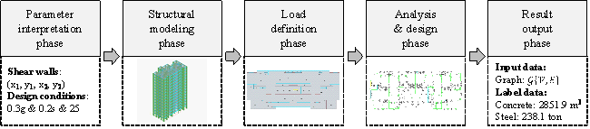
Figure 6. Parametric modeling procedure
6 Alternative CMQ estimation modeling options
Three existing neural network architectures are utilized to establish the CMQ estimation models. Their capacities have been validated in either CMQ estimation or shear wall building structure-related design tasks, and are therefore served as benchmarks. These neural network estimation models are then compared with the proposed Graph-GEN in Section 7 to demonstrate the superiority of the latter.
6.1 ANN
One of the most widely
used models for CMQ estimation tasks is ANN (Table 1). This model, also referred
to as a multilayer perceptron (MLP), includes several fully connected layers
and adopts dropout and batch normalization techniques. Based on the characteristics
of an RC shear wall building structure, nine input features are selected: total
length of the shear walls, total length of the beams, average thickness of the
shear walls, average height of the beams, floor area, floor height, number of
floors ( ![]() ), design seismic acceleration (
), design seismic acceleration ( ![]() ), and site characteristic period (
), and site characteristic period ( ![]() ).
).
6.2 CNN
CNN is a widely used architecture
in computer vision. To fit the input form of the CNN, the structural design
(shear wall and beam layout shown in Figure 2(a)) and the design conditions
are represented as a six-channel pixel image (i.e., a 512 ˇÁ 256 ˇÁ 6 matrix).
For each channel (i.e., a 512 ˇÁ 256 matrix), a nonzero element indicates that
a structural component exists at this position, whereas a zero element indicates
otherwise (Fei et al., 2022a). The values of the nonzero elements in the six
channels represent the component width, component height, number of floors (
![]() ), design seismic acceleration (
), design seismic acceleration ( ![]() ), site characteristic period (
), site characteristic period ( ![]() ), and scale factor (to scale the structural design into a 512 ˇÁ 256 matrix).
A classical CNN model, ResNet (He et al., 2016), is selected to establish the
mapping relationship between the input matrix and CMQ vector. ResNet has been
proven successful in its application to the seismic response prediction of RC
shear wall building structures, indicating its potential in investigating structural
design-related problems (Lu et al., 2022).
), and scale factor (to scale the structural design into a 512 ˇÁ 256 matrix).
A classical CNN model, ResNet (He et al., 2016), is selected to establish the
mapping relationship between the input matrix and CMQ vector. ResNet has been
proven successful in its application to the seismic response prediction of RC
shear wall building structures, indicating its potential in investigating structural
design-related problems (Lu et al., 2022).
6.3 GNN
An existing GNN model, Graph-SF, is also used for comparison (Zhao et al., 2023a). This model considers edge features in the feature aggregation process. Compared with the classical GCN (Kipf & Welling, 2016) and Graph-SAGE (Hamilton et al., 2018), Graph-SF is more suitable for tasks focusing on edges and has been successfully applied to shear wall layout tasks (Zhao et al., 2023b).
The input of Graph-SF
only includes a graph and the corresponding node and edge features. Therefore,
the global features are considered as part of the edge features (that is, the
edge features are six-dimensional vectors (component length, component width,
component height, ![]() ,
, ![]() , and
, and ![]() )). The output of Graph-SF is a vector representation of each edge.
The output layer is modified such that it is applicable to CMQ estimation. Similar
to Graph-GEN, the vector representations of all the edges are summed and mapped
into one vector through fully connected layers (Algorithm 2). This vector represents
the whole graph and is therefore considered the target CMQ estimation.
)). The output of Graph-SF is a vector representation of each edge.
The output layer is modified such that it is applicable to CMQ estimation. Similar
to Graph-GEN, the vector representations of all the edges are summed and mapped
into one vector through fully connected layers (Algorithm 2). This vector represents
the whole graph and is therefore considered the target CMQ estimation.
As demonstrated above, Graph-SF is less suitable for CMQ estimation than Graph-GEN. The deficiency in Graph-SF architecture results in mixed global and edge features, which causes information redundancy during feature aggregation in GNN layers. Additionally, Graph-SF fails to take prior knowledge into consideration.
7 Numerical experiments and discussions
Numerical experiments are performed on a personal computer with an NVIDIA GeForce RTX 3090 GPU and an Intel Core i7-10700K CPU @ 3.80 GHz. Both StructGAN and Graph-GEN are implemented in the PyTorch deep learning framework (PyTorch, 2023) and trained on a GPU. Graphs are created using the Deep Graph Library (DGL, 2023). Through a secondary development, the parametric modeling procedure of the RC shear wall building structure is established using the structural design software YJK-GAMA (YJK, 2023) and executed on the CPU. YJK is one of the most widely used structural design programs in China. Its reinforcement design and material consumption results are those typically accepted by structural engineers.
Data augmentation is performed, as described in Section 5. The training strategy and hyperparameter selection for StructGAN have been described in Liao et al. (2022). The trained StructGAN and established parametric modeling procedure are applied to a structural design dataset with 430 cases, as described in Section 5.1. Note that the dataset is split into training (80%) and testing (20%) sets before data augmentation. To train the CMQ estimation models, a five-fold cross-validation is adopted. The optimizer used is Adam (Kingma & Ba, 2017), which had a learning rate of 0.001 and a weight decay of 0.0001. The batch size and number of epochs are 8 and 100, respectively. The prediction results of the five CMQ estimation models (from the five-fold cross-validation) are averaged to improve the performance stability.
The widely used MAPE and standard deviation of absolute percentage error (SDAPE) are used as evaluation metrics for the CMQ estimation models (Garc¨Şa de Soto et al., 2015; Wang et al., 2016). They can be calculated using Equations (12)¨C(14):
|
|
(12) |
|
|
|
(13) |
|
|
|
(14) |
where ![]() is the averaged CMQ estimated by the five estimation models;
is the averaged CMQ estimated by the five estimation models;
![]() is the accurate CMQ; and
is the accurate CMQ; and ![]() is the number of samples.
is the number of samples.
The hyperparameters of data-driven models are selected based on the MAPE and SDAPE in the following sections.
7.1 Discussion on data-driven modeling options
Several data-driven modelsˇŞMLP,
ResNet, Graph-SF, and Graph-GENˇŞare trained and tested on the CMQ dataset. Each
model had three variants each having a different number of layers ( ![]() ), as shown in Table 3. For GNN models, K=M=
), as shown in Table 3. For GNN models, K=M= ![]() , where K is the graph depth in Algorithm 1 and M is
the number of fully connected layers in Algorithm 2; N=
, where K is the graph depth in Algorithm 1 and M is
the number of fully connected layers in Algorithm 2; N= ![]() , where N is the number of fully connected layers in Algorithm
3;
, where N is the number of fully connected layers in Algorithm
3; ![]() is selected as the nonlinear activation function
is selected as the nonlinear activation function ![]() in Algorithms 1-3; knowledge inclusion is
neglected, i.e.,
in Algorithms 1-3; knowledge inclusion is
neglected, i.e., ![]() (see Section 4.3 for details). Based on the CMQ dataset,
(see Section 4.3 for details). Based on the CMQ dataset,
![]() and
and ![]() =1.3 (Equations 8 and 9). Details of Graph-GEN architecture can be
found in Appendix B.
=1.3 (Equations 8 and 9). Details of Graph-GEN architecture can be
found in Appendix B.
The model performance values on the test set are shown in Table 3. The prediction accuracies of MLP and ResNet are similar, with concrete MAPE ranging from 5.2% to 6.8% and steel MAPE ranging from 10.8% to 12.2%. In contrast, GNN models exhibit significantly improved performance, with concrete MAPE ranging from 2.3% to 3.2% and steel MAPE ranging from 8.6% to 9.5%. This improvement can be attributed to GNNˇŻs ability to extract features in topology (component layout) more effectively than CNN and ANN. Additionally, Graph-GEN outperforms Graph-SF in the estimation accuracy of both concrete and steel, indicating the proposed architectureˇŻs superior capacity in handling heterogeneous data. Overall, the six-layer Graph-GEN architecture achieves the lowest MAPE (2.3% for concrete and 8.6% for steel) and SDAPE (1.8% for concrete and 7.3% for steel) and will be used in subsequent experiments.
Table 3. Performance of different data-driven modeling options on CMQ test set
|
Data-driven model |
|
Concrete |
Steel |
||
|
MAPE (%) |
SDAPE (%) |
MAPE (%) |
SDAPE (%) |
||
|
MLP (Garc¨Şa de Soto et al., 2015) |
3 |
5.2 |
5.7 |
11.1 |
8.1 |
|
5 |
6.8 |
7.7 |
12.2 |
9.7 |
|
|
7 |
6.0 |
6.2 |
11.0 |
8.5 |
|
|
ResNet (Lu et al., 2022) |
18 |
5.6 |
5.9 |
10.8 |
9.0 |
|
50 |
5.5 |
5.3 |
10.8 |
9.0 |
|
|
101 |
6.0 |
6.8 |
11.4 |
9.4 |
|
|
Graph-SF (Zhao et al., 2023a) |
4 |
2.7 |
2.2 |
9.3 |
7.2 |
|
6 |
2.6 |
2.0 |
9.5 |
7.3 |
|
|
8 |
3.2 |
2.5 |
9.5 |
7.5 |
|
|
Graph-GEN |
4 |
2.5 |
2.0 |
8.6 |
7.3 |
|
6 |
2.3 |
1.8 |
8.6 |
7.3 |
|
|
8 |
3.1 |
2.4 |
9.2 |
7.4 |
|
7.2 Discussion on feature representation options
The representation details of the input and output features are further discussed based on the six-layer Graph-GEN. The input features are either normalized or scaled, as given by Equations (15) and (16):
|
|
(15) |
|
|
|
(16) |
where ![]() is the normalized input feature;
is the normalized input feature; ![]() is the original input feature (for coordinates, assuming
that the center coordinates are at the origin (Zhao et al., 2023b));
is the original input feature (for coordinates, assuming
that the center coordinates are at the origin (Zhao et al., 2023b)); ![]() and
and ![]() are the mean and standard deviation of
are the mean and standard deviation of ![]() , respectively;
, respectively; ![]() is the scaled input feature; and
is the scaled input feature; and ![]() is the scale factor such that
is the scale factor such that ![]() . For the coordinates, length, width, and height,
. For the coordinates, length, width, and height, ![]() ; for
; for ![]() ,
, ![]() ; and for
; and for ![]() and
and ![]() ,
, ![]() .
.
The output features adopt one of the following CMQ vectors: (1) two-dimensional vector, i.e., noutput=2 in Appendix B, representing the combined quantity of concrete and steel and (2) six-dimensional vector, i.e., noutput=6 in Appendix B, representing the separated quantities of concrete and steel for shear walls, beams, and slabs. These two CMQ vectors are normalized.
The experimental results using different feature representations are given in Table 4. It can be observed that the output feature type (combined or separated) has a minor impact on the estimation accuracy for a given input feature type (normalized or scaled), with a maximum variation in MAPE of 0.4% (i.e., 3.2%-2.8%). However, for a given output feature type, the normalized input feature yields better estimation accuracy than the scaled input feature, with up to 1% (i.e., 9.6%-8.6%) improvement in MAPE. The model with normalized input features and combined output features achieves the lowest MAPE and SDAPE for both concrete and steel. Thus, these options are chosen for subsequent experiments.
Table 4. Performance of different feature representation options on CMQ test set
|
Input feature |
Output feature |
Concrete |
Steel |
||
|
MAPE (%) |
SDAPE (%) |
MAPE (%) |
SDAPE (%) |
||
|
Normalized |
Combined |
2.3 |
1.8 |
8.6 |
7.3 |
|
Scaled |
Combined |
3.2 |
2.8 |
9.6 |
7.4 |
|
Normalized |
Separated |
2.4 |
2.0 |
8.9 |
7.3 |
|
Scaled |
Separated |
3.4 |
3.2 |
9.2 |
7.3 |
7.3 Discussion on knowledge inclusion strategies
The hyperparameters for knowledge inclusion are further tuned based on the best, purely data-driven model. The model performance values on the test set are listed in Table 5. They are elaborated as follows.
(1) When ![]() , the model is purely data-driven through the loss function
, the model is purely data-driven through the loss function
![]() .
.
(2) When ![]() , prior knowledge only controls the model through the loss function
, prior knowledge only controls the model through the loss function
![]() . The predictions of the model cannot be guaranteed to fully satisfy
the prior knowledge. As listed in Table 5, the MAPE is increased by a minimum
of 0.1% (i.e., 2.4%-2.3%) and a maximum of 0.7% (i.e., 9.3%-8.6%) because of
the interference of the two loss functions (i.e.,
. The predictions of the model cannot be guaranteed to fully satisfy
the prior knowledge. As listed in Table 5, the MAPE is increased by a minimum
of 0.1% (i.e., 2.4%-2.3%) and a maximum of 0.7% (i.e., 9.3%-8.6%) because of
the interference of the two loss functions (i.e., ![]() and
and ![]() ).
).
(3) When ![]() , the model directly replaces the erroneous prediction results at the output
layer to ensure that the prior knowledge is 100% satisfied; meanwhile, the corresponding
gradient in
, the model directly replaces the erroneous prediction results at the output
layer to ensure that the prior knowledge is 100% satisfied; meanwhile, the corresponding
gradient in ![]() disappears. In this case, the model parameters related to
the incorrect prediction are updated through
disappears. In this case, the model parameters related to
the incorrect prediction are updated through ![]() to a certain extent (depending on the
to a certain extent (depending on the
![]() value). It can be observed that when
value). It can be observed that when ![]() , the MAPE and SDAPE values of concrete are 30.4% and 38.9% smaller
relative to those of the purely data-driven model, respectively. Regretfully,
the MAPE of steel increases by 2.3% relatively, and its SDAPE remains unchanged.
, the MAPE and SDAPE values of concrete are 30.4% and 38.9% smaller
relative to those of the purely data-driven model, respectively. Regretfully,
the MAPE of steel increases by 2.3% relatively, and its SDAPE remains unchanged.
The
results obtained when ![]() imply that the maximum concrete consumption can effectively
govern the model prediction, whereas, in general, minimum steel consumption
is unable to provide useful information. This is due to the fact that in the
CMQ dataset used in this study, the minimum steel consumption is only about
2/3 of the actual steel consumption (label) calculated by commercial design
software. Since the minimum bound is relatively low, this prior knowledge is
only beneficial at the beginning of the training when the error is huge. Nevertheless,
the minimum steel consumption can still be used to prevent the model from producing
major errors under certain circumstances (see Section 8.2).
imply that the maximum concrete consumption can effectively
govern the model prediction, whereas, in general, minimum steel consumption
is unable to provide useful information. This is due to the fact that in the
CMQ dataset used in this study, the minimum steel consumption is only about
2/3 of the actual steel consumption (label) calculated by commercial design
software. Since the minimum bound is relatively low, this prior knowledge is
only beneficial at the beginning of the training when the error is huge. Nevertheless,
the minimum steel consumption can still be used to prevent the model from producing
major errors under certain circumstances (see Section 8.2).
Table 5. Performance of different knowledge inclusion strategies on CMQ test set
|
|
|
Concrete |
Steel |
||
|
MAPE (%) |
SDAPE (%) |
MAPE (%) |
SDAPE (%) |
||
|
0 |
0 |
2.3 |
1.8 |
8.6 |
7.3 |
|
0 |
0.01 |
2.5 |
2.4 |
9.2 |
7.2 |
|
0 |
0.1 |
2.6 |
2.5 |
9.3 |
7.2 |
|
0 |
1 |
2.4 |
1.8 |
9.2 |
7.3 |
|
1 |
0.01 |
2.0 |
1.0 |
8.8 |
7.3 |
|
1 |
0.1 |
1.6 |
1.1 |
8.8 |
7.3 |
|
1 |
1 |
1.8 |
1.4 |
9.0 |
7.2 |
Note that Graph-GEN has low computational requirements and good scalability. All Graph-GEN configurations described in this section use less than 2GB GPU memory during training. The saved Graph-GEN models are smaller than 1GB and can run on any consumer grade CPU.
8 Case study
To verify the effectiveness of the proposed method, a trained Graph-GEN is applied in the structural design of three typical shear wall structures of residential buildings and results are compared with existing CMQ estimation methods. Residential buildings with seismic intensity, site condition, floor area, and number of floors considered in this case study are commonly built in China.
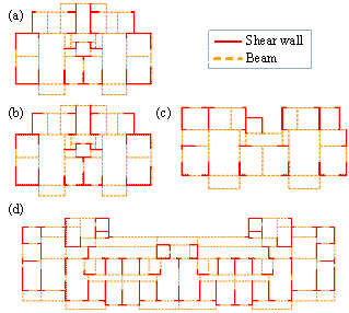
Figure 7. Structural design schemes of shear wall structures of residential buildings: (a) scheme ˘ń of Building A; (b) scheme ˘ň of Building A; (c) Building B; (d) Building C.
8.1 Comparison of alternative design schemes
During the structural design of shear wall structures of residential buildings, various design schemes may be proposed and compared to obtain an optimal one. In this case study, the material cost and carbon emission of two design schemes of Building A are estimated and compared to guide the direction of design optimization.
Essential information
of the project is given below. Building A has 11 floors, and each has a floor
area of 220 m2. The seismic intensity is 7 degrees ( ![]() ), the site is class II, and the seismic design group is 2 (
), the site is class II, and the seismic design group is 2 (
![]() ). The structural layouts of the two design schemes with different
shear-wall lengths are shown in Figures 7(a) and 7(b). The shear-wall thicknesses
are both 180 mm. The underground structure is not considered in this study.
). The structural layouts of the two design schemes with different
shear-wall lengths are shown in Figures 7(a) and 7(b). The shear-wall thicknesses
are both 180 mm. The underground structure is not considered in this study.
A refined finite element model of the building is established using the parametric modeling procedure (see Section 5.3) in the structural design software YJK-GAMA (see Section 7). Structural analysis and reinforcement design are performed, and the obtained CMQs are considered as the ground truth. An MLP, a Graph-SF, a Graph-GEN, and a simplified method are used to estimate the CMQs. Each data-driven model adopts the best configuration listed in Tables 3-5, according to MAPEs. Specifically, the simplified method considers the calculated volume of all structural components as concrete consumption, and assumes the reinforcement ratio as 0.1-ton steel per 1 m3 concrete, which is an empirical ratio obtained from the training dataset explained in Section 5.1. Based on the CMQs, material cost, and carbon emission are calculated based on ChinaˇŻs statistical data (Zhang & Zhang, 2021). Assuming 1 USD = 7 CNY. For C35 concrete, the unit cost is 544 CNY/m3 (~78 USD/m3) and the unit emission is 387 kgCO2e/m3. For HRB400 steel, the averaged cost is 6266 CNY/ton (~895 USD/ton) and the averaged emission is 2262 kgCO2e/ton. Comparisons of the estimation accuracy of CMQ, and material cost and carbon emission by different methods are summarized in Tables 6 and 7, respectively.
It can be concluded from Table 6 that the CMQ error of the simplified method ranges from 6.5% to 24.1%, that of MLP ranges from -2.3% to 13.8%, that of Graph-SF ranges from -2.2% to 1.7%, and that of Graph-GEN ranges from -0.7% to 1.9%. It can also be determined from Table 7 that the cost and emission error of the simplified method ranges from 11.9% to 15.3%, that of MLP ranges from 1.0% to 8.9%, that of Graph-SF ranges from -1.9% to 0.3%, and that of Graph-GEN ranges from 0.3% to 1.0%. Therefore, the proposed Graph-GEN has a significant accuracy advantage over Graph-SF, MLP, and the simplified method.
In terms of time efficiency, the times used for a single CMQ estimation are: ~3 minutes (YJK); 0.36 seconds (Graph-GEN); 0.35 seconds (Graph-SF); 0.19 seconds (MLP); ~0.001 seconds (simplified method). It can be observed that the proposed Graph-GEN is remarkably advantageous (an increase of 500 times), over YJK, which calculates the CMQs of each structural component after detailed structural analysis and reinforcement design. When using genetic algorithms for structural optimization, hundreds of times of CMQ estimation are typically needed (Zhou et al., 2022; Orhan & Taşkın, 2021). For example, a population size of 20 and an iteration number of 50 will result in 1000 possible schemes and 1000 times of CMQ estimation. If YJK is used, CMQ estimation alone will take 50 hours, which is unacceptable for urgent design tasks. However, if Graph-GEN is used, CMQ estimation will only take 6 minutes and will not cause a bottleneck for structural optimization. Although Graph-GEN is not the quickest method, its efficiency and accuracy can well satisfy the needs of engineering practices.
Therefore, the proposed method demonstrates a highly desirable balance between accuracy and efficiency.
8.2 Advantages of knowledge inclusion
In this case study, the CMQ estimations by different methods are compared with the maximum concrete consumption and the minimum steel consumption according to the prior knowledge specified in Section 4.3.
Essential information
of the two projects is given below. Building B has 8 floors, and each has a
floor area of 210 m2. Building C has 25 floors, and each has a floor
area of 800 m2. They are both considered for a seismic intensity
of 8 degrees ( ![]() ), a site class of II, and a seismic design group of 2 (
), a site class of II, and a seismic design group of 2 ( ![]() ). The structural layouts of the two buildings are shown in Figures
7(c) and 7(d). The shear-wall thicknesses of Buildings B and C are 180 mm and
240 mm, respectively. The underground structure is not considered herein.
). The structural layouts of the two buildings are shown in Figures
7(c) and 7(d). The shear-wall thicknesses of Buildings B and C are 180 mm and
240 mm, respectively. The underground structure is not considered herein.
The CMQs of Buildings
B and C are estimated using the five methods in Section 8.1. The maximum concrete
consumption ( ![]() ) of Building B is calculated as 68.0 m3 per floor, and
the minimum steel consumption (
) of Building B is calculated as 68.0 m3 per floor, and
the minimum steel consumption ( ![]() ) of Building C is calculated as 25.7 tons per floor. A comparison
of the prior knowledge and the CMQ estimated by different methods is summarized
in Table 8.
) of Building C is calculated as 25.7 tons per floor. A comparison
of the prior knowledge and the CMQ estimated by different methods is summarized
in Table 8.
For Building B, the concrete usages estimated by the simplified method, MLP, and Graph-SF are larger than the maximum concrete consumption, whereas only the concrete usage estimated by Graph-GEN satisfies the prior knowledge. For Building C, the steel usages estimated by MLP and Graph-SF are smaller than the minimum steel consumption. In contrast, steel usage estimated by Graph-GEN satisfies the prior knowledge. This case study shows that the proposed prior knowledge inclusion strategy can effectively avoid the fundamental errors that might be encountered by existing data-driven methods.
Table 6. CMQ estimation accuracy of different methods (per floor)
|
Method |
Scheme ˘ń of Building A |
Scheme ˘ň of Building A |
||||||
|
Concrete (m3) |
Percentage error (%) |
Steel (ton) |
Percentage error (%) |
Concrete (m3) |
Percentage error (%) |
Steel (ton) |
Percentage error (%) |
|
|
YJK |
74.0 |
0.0 |
6.5 |
0.0 |
75.1 |
0.0 |
6.4 |
0.0 |
|
Simplified |
78.9 |
6.6 |
7.9 |
22.3 |
79.9 |
6.5 |
8.0 |
24.1 |
|
MLP |
72.3 |
-2.3 |
6.9 |
7.4 |
78.1 |
4.0 |
7.3 |
13.8 |
|
Graph-SF |
72.8 |
-1.6 |
6.3 |
-2.2 |
74.2 |
-1.1 |
6.5 |
1.7 |
|
Graph-GEN |
74.9 |
1.3 |
6.4 |
-0.7 |
75.1 |
0.1 |
6.6 |
1.9 |
Table 7. Cost and emission estimation accuracy of different methods (per floor)
|
Method |
Scheme ˘ń of Building A |
Scheme ˘ň of Building A |
||||||
|
Cost (USD) |
Percentage error (%) |
Emission (kgCO2e) |
Percentage error (%) |
Cost (USD) |
Percentage error (%) |
Emission (kgCO2e) |
Percentage error (%) |
|
|
YJK |
11546.4 |
0.0 |
43232.5 |
0.0 |
11617.4 |
0.0 |
43611.4 |
0.0 |
|
Simplified |
13214.7 |
14.4 |
48377.7 |
11.9 |
13390.7 |
15.3 |
49022.0 |
12.4 |
|
MLP |
11841.3 |
2.6 |
43655.9 |
1.0 |
12649.4 |
8.9 |
46793.1 |
7.3 |
|
Graph-SF |
11324.6 |
-1.9 |
42442.4 |
-1.8 |
11648.4 |
0.3 |
43530.6 |
-0.2 |
|
Graph-GEN |
11582.8 |
0.3 |
43504.2 |
0.6 |
11731.8 |
1.0 |
43908.1 |
0.7 |
Table 8. Influence of knowledge inclusion on CMQ estimations (per floor)
|
Method |
Building B |
Building C |
||||
|
Concrete (m3) |
Percentage error (%) |
Knowledge satisfied? |
Steel (ton) |
Percentage error (%) |
Knowledge satisfied? |
|
|
YJK |
67.3 |
0.0 |
Yes |
28.2 |
0.0 |
Yes |
|
Simplified |
71.6 |
6.4 |
No |
33.4 |
18.4 |
Yes |
|
MLP |
72.7 |
8.0 |
No |
22.0 |
-22.1 |
No |
|
Graph-SF |
72.3 |
7.4 |
No |
23.6 |
-16.3 |
No |
|
Graph-GEN |
68.0 |
1.1 |
Yes |
25.7 |
-8.9 |
Yes |
Note: The maximum concrete consumption of Building B is 68.0 m3 per floor and the minimum steel consumption of Building C is 25.7 ton per floor.
9 Conclusion
This study proposes an accurate and efficient CMQ estimation method for RC buildings. The major contributions are as follows. First, a data augmentation method is proposed for the CMQ dataset, incorporating GANs and parametric modeling. Second, a novel GNN architecture, Graph-GEN, is constructed to enable feature extraction and fusion of heterogeneous data, including component layout (topology), component section sizes (geometry), and design conditions (text). Third, prior knowledge is introduced into Graph-GEN to further improve the model accuracy and thus prevent potential major and fundamental errors. The following specific conclusions are also drawn.
(1) Through the unique cooperation of GANs and parametric modeling, synthetic structural designs can be effectively generated and CMQs can be automatically calculated, thereby enlarging the data size by 10 times, which greatly facilitate the training of the CMQ estimation model.
(2) The heterogeneous feature fusion mechanism of the proposed Graph-GEN architecture can facilitate accurate mapping between the input information and CMQs. Graph-GEN is significantly superior to the existing ANN, CNN, and GNN methods in terms of MAPE and SDAPE. These strongly convey the novelty of this study.
(3) Unlike the existing studies, by modifying the loss function and output layer in the present study, the proposed knowledge inclusion strategy can further reduce the MAPE and SDAPE of concrete consumption by 30.4% and 38.9%, respectively. Notably, it can ensure that the estimated steel consumption exceeds the minimum steel consumption required by the design codes.
(4) The case study shows that Graph-GEN outperforms three existing methods in terms of estimation accuracy, and is 500 times more efficient than the commercial design software. It also demonstrates the advantages of knowledge inclusion in avoiding fundamental errors. To this end, Graph-GEN exhibits a highly desirable balance between computational accuracy and efficiency.
The limitations of this study are recognized as: (1) the minimum reinforcement requirement embedded in the Graph-GEN is a simplification to the complex reinforcement design; (2) the influence of the underground structures on CMQs is ignored. In the future study, Graph-GEN shall incorporate more domain knowledge to improve its practicality. Further, it should be applied in the evaluation stage of evolutionary algorithms and deep learning models to explore its applicability.
AppendIx a
The seismic design condition
is represented by the design seismic acceleration, ![]() , which corresponds to a 10% probability of exceedance over 50 years.
, which corresponds to a 10% probability of exceedance over 50 years.
The site design condition
is represented by the site characteristic period, ![]() , as listed in Table A1.
, as listed in Table A1.
The height design condition
is represented by the number of superstructure floors, ![]() , excluding the underground floors, which are not considered in this
study.
, excluding the underground floors, which are not considered in this
study.
Table A1. Site characteristic period (s) (MOHURD, 2016)
|
Seismic design group |
Site class |
||||
|
˘ń0 |
˘ń1 |
˘ň |
˘ó |
˘ô |
|
|
1 |
0.20 |
0.25 |
0.35 |
0.45 |
0.65 |
|
2 |
0.25 |
0.30 |
0.40 |
0.55 |
0.75 |
|
3 |
0.30 |
0.35 |
0.45 |
0.65 |
0.90 |
AppendIx B
Details of Graph-GEN architecture are listed in Table B1. According to the feature representation outlined in Section 4.1, nnode = 2, nedge = 3, and nglobal = 3. According to the output feature type in Section 7.2, noutput =2 or 6. The dropout ratio (p) is 0.2, and the nonlinear activation function (¦Ň(ˇ¤)) adopts ReLU(ˇ¤).
Each GNNLayer(nnode,in, nedge,in, nnode,out) consists of two weighting matrices: Linear(2ˇÁnnode,in + nedge,in, nnode,out) and Linear(nnode,in + nnode,out, nnode,out), see Algorithm 1.
Table B1. Architecture of GNN models
|
Parameters |
Architecture |
|
K=4 M=4 N=1 |
GNNLayer(nnode, nedge, 8); Dropout(p); GNNLayer(8, nedge, 8); Dropout(p); BatchNorm(8); Dropout(p); GNNLayer(8, nedge, 16); Dropout(p); GNNLayer(16, nedge, 16); ¦Ň(Linear(32 + nedge, 64)); ¦Ň(Linear(64, 64)); BatchNorm(64); Dropout(p); ¦Ň(Linear(64, 32)); ¦Ň(Linear(32, 8)); ¦Ň(Linear(8, 8)); ¦Ň(Linear(nglobal, 8)); Linear(16, noutput) |
|
K=6 M=6 N=2 |
GNNLayer(nnode, nedge, 8); Dropout(p); GNNLayer(8, nedge, 8); Dropout(p); BatchNorm(8); Dropout(p); GNNLayer(8, nedge, 16); Dropout(p); GNNLayer(16, nedge, 16); Dropout(p); BatchNorm(16); Dropout(p); GNNLayer(16, nedge, 32); Dropout(p); GNNLayer(32, nedge, 32); ¦Ň(Linear(64 + nedge, 128)); ¦Ň(Linear(128, 128)); BatchNorm(128); Dropout(p); ¦Ň(Linear(128, 64)); ¦Ň(Linear(64, 64)); BatchNorm(64); Dropout(p); ¦Ň(Linear(64, 32)); ¦Ň(Linear(32, 8)); ¦Ň(Linear(8, 8)); ¦Ň(Linear(nglobal, 8)); ¦Ň(Linear(16, 8)); Linear(8, noutput) |
|
K=8 M=8 N=3 |
GNNLayer(nnode, nedge, 8); Dropout(p); GNNLayer(8, nedge, 8); Dropout(p); BatchNorm(8); Dropout(p); GNNLayer(8, nedge, 16); Dropout(p); GNNLayer(16, nedge, 16); Dropout(p); BatchNorm(16); Dropout(p); GNNLayer(16, nedge, 32); Dropout(p); GNNLayer(32, nedge, 32); Dropout(p); BatchNorm(32); Dropout(p); GNNLayer(32, nedge, 64); Dropout(p); GNNLayer(64, nedge, 64); ¦Ň(Linear(128 + nedge, 256)); ¦Ň(Linear(256, 256)); BatchNorm(256); Dropout(p); ¦Ň(Linear(256, 128)); ¦Ň(Linear(128, 128)); BatchNorm(128); Dropout(p); ¦Ň(Linear(128, 64)); ¦Ň(Linear(64, 64)); BatchNorm(64); Dropout(p); ¦Ň(Linear(64, 32)); ¦Ň(Linear(32, 8)); ¦Ň(Linear(8, 8)); ¦Ň(Linear(nglobal, 8)); ¦Ň(Linear(16, 8)); ¦Ň(Linear(8, 4)); Linear(4, noutput) |
ApPENDIX C
For shear walls, the minimum reinforcement within the end restraint zone and the minimum reinforcement ratio of the wall distribution rebars are listed in Tables C1 and C2, respectively.
Table C1. Minimum reinforcement within end restraint zone (MOHURD, 2010)
|
Seismic grade |
Minimum longitudinal bars |
Minimum tie bar diameter (mm) |
Maximum vertical spacing of tie bars (mm) |
|
1 |
Max(0.008
|
8 |
150 |
|
2 |
Max(0.006
|
8 |
200 |
|
3 |
Max(0.005
|
6 |
200 |
|
4 |
Max(0.004
|
6 |
250 |
Note: ![]() is the section area of the end restraint zone;
is the section area of the end restraint zone; ![]() denotes rebar diameter.
denotes rebar diameter.
Table C2. Minimum reinforcement ratio of wall distribution rebars (MOHURD, 2016)
|
Seismic grade |
Minimum reinforcement ratio of horizontal and vertical wall distribution rebars |
|
1 |
0.25% |
|
2 |
0.25% |
|
3 |
0.25% |
|
4 |
0.20% |
For beams (including frame beams and coupling beams), the minimum requirements of the longitudinal tensile rebars, erecting rebars, and stirrups are listed in Tables C3¨CC6.
Table C3. Minimum reinforcement ratio of longitudinal tensile rebars of frame beams (MOHURD, 2010)
|
Seismic grade |
Beam end (%) |
Beam midspan (%) |
|
1 |
Max(0.40, 80
|
Max(0.30, 65
|
|
2 |
Max(0.30, 65
|
Max(0.25, 55
|
|
3 or 4 |
Max(0.25, 55
|
Max(0.20, 45
|
Note: ![]() is the tensile strength of concrete, and
is the tensile strength of concrete, and ![]() is the yield strength of steel rebar.
is the yield strength of steel rebar.
Table C4. Minimum reinforcement ratio of longitudinal tensile rebars of coupling beams (MOHURD, 2010)
|
Span¨Cdepth ratio |
Minimum reinforcement ratio (%) |
|
|
Max(0.20, 45
|
|
|
Max(0.25, 55
|
Note: ![]() is the tensile strength of concrete, and
is the tensile strength of concrete, and ![]() is the yield strength of steel rebar.
is the yield strength of steel rebar.
Table C5. Minimum erecting rebars (MOHURD, 2015)
|
Seismic grade |
Minimum number of rebars at top and bottom |
Minimum rebar diameter (mm) |
|
1 or 2 |
2 |
14 |
|
3 or 4 |
2 |
12 |
Table C6. Minimum stirrups in beams (MOHURD, 2010)
|
Seismic grade |
Length of dense zone (mm) |
Maximum spacing of stirrups (mm) |
Minimum stirrup diameter (mm) |
|
1 |
Max(2 |
Max( |
10 |
|
2 |
Max(1.5 |
Max( |
8 |
|
3 |
Max(1.5 |
Max( |
8 |
|
4 |
Max(1.5 |
Max( |
6 |
Note: ![]() is the beam section height, and d is the longitudinal rebar
diameter.
is the beam section height, and d is the longitudinal rebar
diameter.
For slabs, the minimum
reinforcement ratio (%) of the longitudinal tensile rebars is Max(0.20, 45
![]() ). (MOHURD, 2015).
). (MOHURD, 2015).
ACKNOWLEDGMENT
Adeli, H. (2020). Four decades of computing in civil engineering. In CIGOS 2019, Innovation for Sustainable Infrastructure: Proceedings of the 5th International Conference on Geotechnics, Civil Engineering Works and Structures (pp. 3-11). Springer Singapore.
Adeli, H., & Kim, H. (2001). Cost optimization of composite floors using neural dynamics model. Communications in numerical methods in engineering, 17(11), 771-787.
Adeli, H., & Sarma, K. (2006). Cost Optimization of Structures ¨C Fuzzy Logic, Genetic Algorithms, and Parallel Computing, John Wiley and Sons, West Sussex, United Kingdom.
Adeli, H., & Wu, M. (1998). Regularization Neural Network for Construction Cost Estimation. Journal of Construction Engineering and Management, 124(1), 18¨C24.
Afzal, M., Liu, Y., Cheng, J. C. P., & Gan, V. J. L. (2020). Reinforced concrete structural design optimization: A critical review. Journal of Cleaner Production, 260, 120623.
Ahmadkhanlou, F., & Adeli, H. (2005). Optimum cost design of reinforced concrete slabs using neural dynamics model. Engineering Applications of Artificial Intelligence, 18(1), 65-72.
Aldwaik, M., & Adeli, H. (2014). Advances in optimization of highrise building structures. Structural and Multidisciplinary Optimization, 50(6), 899¨C919.
Aldwaik, M., & Adeli, H. (2016). Cost optimization of reinforced concrete flat slabs of arbitrary configuration in irregular highrise building structures. Structural and Multidisciplinary Optimization, 54, 151-164.
Ampanavos, S., Nourbakhsh, M., & Cheng, C.-Y. (2022). Structural Design Recommendations in the Early Design Phase Using Machine Learning. In D. Gerber, E. Pantazis, B. Bogosian, A. Nahmad, & C. Miltiadis (Eds.), Computer-Aided Architectural Design. Design Imperatives: The Future is Now (pp. 190¨C202). Springer.
Antoniou, F., Aretoulis, G., Giannoulakis, D., & Konstantinidis, D. (2023). Cost and Material Quantities Prediction Models for the Construction of Underground Metro Stations. Buildings, 13(2), Article 2.
Beljkaš, Ž., Knežević, M., Rutešić, S., & Ivanišević, N. (2020). Application of Artificial Intelligence for the Estimation of Concrete and Reinforcement Consumption in the Construction of Integral Bridges. Advances in Civil Engineering, 2020, e8645031.
Boscardin, J. T., Yepes, V., & Kripka, M. (2019). Optimization of reinforced concrete building frames with automated grouping of columns. Automation in Construction, 104, 331¨C340.
Bubeck, S., Chandrasekaran, V., Eldan, R., Gehrke, J., Horvitz, E., Kamar, E., Lee, P., Lee, Y. T., Li, Y., Lundberg, S., Nori, H., Palangi, H., Ribeiro, M. T., & Zhang, Y. (2023). Sparks of Artificial General Intelligence: Early experiments with GPT-4 (arXiv:2303.12712). arXiv.
Chang, K.-H., & Cheng, C.-Y. (2020). Learning to Simulate and Design for Structural Engineering. Proceedings of the 37th International Conference on Machine Learning, 1426¨C1436.
Che, X., Zheng, Y., Chen, X., Song, S., & Li, S. (2022). Decoding color visual working memory from EEG signals using graph convolutional neural networks. International Journal of Neural Systems, 32(02), 2250003.
Chen, S., Dong, J., Ha, P., Li, Y., & Labi, S. (2021). Graph neural network and reinforcement learning for multi©\agent cooperative control of connected autonomous vehicles. Computer©\Aided Civil and Infrastructure Engineering, 36(7), 838-857.
Chugh, T., Sindhya, K., Hakanen, J., & Miettinen, K. (2019). A survey on handling computationally expensive multiobjective optimization problems with evolutionary algorithms. Soft Computing, 23(9), 3137¨C3166.
DˇŻAmico, B., Myers, R. J., Sykes, J., Voss, E., Cousins-Jenvey, B., Fawcett, W., Richardson, S., Kermani, A., & Pomponi, F. (2019). Machine Learning for Sustainable Structures: A Call for Data. Structures, 19, 1¨C4.
Dash, T., Chitlangia, S., Ahuja, A., & Srinivasan, A. (2022). A review of some techniques for inclusion of domain-knowledge into deep neural networks. Scientific Reports, 12(1), Article 1.
DGL. (2023). Deep Graph Library Tutorials and Documentation. Retrieved from https://docs.dgl.ai/
Dimitriou, L., Marinelli, M., & Fragkakis, N. (2018). Early Bill-of-Quantities Estimation of Concrete Road Bridges: An Artificial Intelligence-Based Application. Public Works Management & Policy, 23(2), 127¨C149.
Du, C., Sun, H., Wang, J., Qi, Q., & Liao, J. (2020). Adversarial and Domain-Aware BERT for Cross-Domain Sentiment Analysis. Proceedings of the 58th Annual Meeting of the Association for Computational Linguistics, 4019¨C4028.
Du, Y., Chen, J., Zhao, C., Liao, F., & Zhu, M. (2022). A hierarchical framework for improving ride comfort of autonomous vehicles via deep reinforcement learning with external knowledge. Computer-Aided Civil and Infrastructure Engineering, 38(8), 1059-1078.
Elfaki, A. O., Alatawi, S., & Abushandi, E. (2014). Using Intelligent Techniques in Construction Project Cost Estimation: 10-Year Survey. Advances in Civil Engineering, 2014, e107926.
El-Sokkary, H., & Galal, K. (2020). Material Quantities of Reinforced Masonry versus Reinforced Concrete Shear Walls. Structures, 27, 767¨C779.
Fan, X., Zhang, X., & Yu, X. (2022). A graph convolution network©\deep reinforcement learning model for resilient water distribution network repair decisions. Computer©\Aided Civil and Infrastructure Engineering, 37(12), 1547-1565.
Fei, Y., Liao, W., Huang, Y., & Lu, X. Z. (2022a). Knowledge-enhanced generative adversarial networks for schematic design of framed tube structures. Automation in Construction, 144, 104619.
Fei, Y., Liao, W., Zhang, S., Yin, P., Han, B., Zhao, P., Chen, X., & Lu, X. Z. (2022b). Integrated Schematic Design Method for Shear Wall Structures: A Practical Application of Generative Adversarial Networks. Buildings, 12(9), Article 9.
Feng, N., Hu, F., Wang, H., & Zhou, B. (2021). Motor intention decoding from the upper limb by graph convolutional network based on functional connectivity. International Journal of Neural Systems, 31(12), 2150047.
Fragkakis, N., Marinelli, M., & Lambropoulos, S. (2015). Preliminary Cost Estimate Model for Culverts. Procedia Engineering, 123, 153¨C161.
Fu, B., Gao, Y., & Wang, W. (2023). Dual generative adversarial networks for automated component layout design of steel frame-brace structures. Automation in Construction, 146, 104661.
Gan, V. J. L., Lo, I. M. C., Ma, J., Tse, K. T., Cheng, J. C. P., & Chan, C. M. (2020). Simulation optimisation towards energy efficient green buildings: Current status and future trends. Journal of Cleaner Production, 254, 120012.
Garc¨Şa de Soto, B., Adey, B. T., & Fernando, D. (2014). A Process for the Development and Evaluation of Preliminary Construction Material Quantity Estimation Models Using Backward Elimination Regression and Neural Networks. Journal of Cost Analysis and Parametrics, 7(3), 180¨C218.
Hamilton, W. L., Ying, R., & Leskovec, J. (2018). Inductive Representation Learning on Large Graphs. arXiv,1706.02216. Retrieved from http://arxiv.org/abs/1706.02216
Hayashi, K., & Ohsaki, M. (2021). Reinforcement learning for optimum design of a plane frame under static loads. Engineering with Computers, 37(3), 1999¨C2011.
He, K., Zhang, X., Ren, S., & Sun, J. (2016). Deep Residual Learning for Image Recognition. 2016 IEEE Conference on Computer Vision and Pattern Recognition (CVPR), 770¨C778.
Idowu, O. S., & Lam, K. C. (2020). Conceptual Quantities Estimation Using Bootstrapped Support Vector Regression Models. Journal of Construction Engineering and Management, 146(4), 04020018.
Jeong, J.-H., & Jo, H. (2021). Deep reinforcement learning for automated design of reinforced concrete structures. Computer-Aided Civil and Infrastructure Engineering, 36(12), 1508¨C1529.
Jin, Y., Wang, H., Chugh, T., Guo, D., & Miettinen, K. (2019). Data-Driven Evolutionary Optimization: An Overview and Case Studies. IEEE Transactions on Evolutionary Computation, 23(3), 442¨C458.
Khan, S., Goucher-Lambert, K., Kostas, K., & Kaklis, P. (2023). ShipHullGAN: A generic parametric modeller for ship hull design using deep convolutional generative model. Computer Methods in Applied Mechanics and Engineering, 411, 116051.
Kim, H., & Adeli, H. (2001). Discrete cost optimization of composite floors using a floating-point genetic algorithm. Engineering Optimization, 33(4), 485-501.
Kim, T.-H., Choi, J.-H., Lee, J.-H., & Shin, H. M. (2013). Performance assessment of hollow RC bridge column sections with reinforcement details for material quantity reduction. Magazine of Concrete Research, 65(21), 1277¨C1292.
Kingma, D. P., & Ba, J. (2017). Adam: A Method for Stochastic Optimization. arXiv, 1412.6980. Retrieved from http://arxiv.org/abs/1412.6980
Kipf, T. N., & Welling, M. (2016). Semi-supervised classification with graph convolutional networks. arXiv, 1609.02907. Retrieved from https://arxiv.org/abs/1609.02907
Kovačević, M., Ivanišević, N., Stević, D., Marković, L. M., Bulajić, B., Marković, L., & Gvozdović, N. (2023). Decision-Support System for Estimating Resource Consumption in Bridge Construction Based on Machine Learning. Axioms, 12(1), Article 1.
Li, S., Snaiki, R., & Wu, T. (2021). A knowledge-enhanced deep reinforcement learning-based shape optimizer for aerodynamic mitigation of wind-sensitive structures. Computer-Aided Civil and Infrastructure Engineering, 36(6), 733¨C746.
Lian, J., & Xu, F. (2022). Spatial enhanced pattern through graph convolutional neural network for epileptic EEG identification. International Journal of Neural Systems, 32(09), 2250033.
Liao, W., Huang, Y., Zheng, Z., & Lu, X. Z. (2022). Intelligent generative structural design method for shear wall building based on ˇ°fused-text-image-to-imageˇ± generative adversarial networks. Expert Systems with Applications, 210, 118530.
Liao, W., Lu, X. Z., Huang, Y., Zheng, Z., & Lin, Y. (2021). Automated structural design of shear wall residential buildings using generative adversarial networks. Automation in Construction, 132, 103931.
Lu, X. Z., Liao, W., Zhang, Y., & Huang, Y. (2022). Intelligent structural design of shear wall residence using physics-enhanced generative adversarial networks. Earthquake Engineering & Structural Dynamics, 51(7), 1657¨C1676.
M¨˘laga-Chuquitaype, C. (2022). Machine Learning in Structural Design: An Opinionated Review. Frontiers in Built Environment, 8, 815717.
Marino, K., Chen, X., Parikh, D., Gupta, A., & Rohrbach, M. (2021). KRISP: Integrating Implicit and Symbolic Knowledge for Open-Domain Knowledge-Based VQA. 14111¨C14121.
MOHURD. (2010). Technical specification for concrete structures of tall building (JGJ 3-2010). China Architecture & Building Press.
MOHURD. (2012). Load Code for the Design of Building Structures (GB50009-2012). China Architecture & Building Press.
MOHURD. (2015). Code for design of concrete structure (GB 50010-2010). China Architecture & Building Press.
MOHURD. (2016). Code for the Seismic Design of Buildings (GB50011-2010). China Architecture & Building Press.
Orhan, T., & Taşkın, K. (2021). Automated topology design of high©\rise diagrid buildings by genetic algorithm optimization. The structural design of tall and special buildings, 30(9), e1853.
Pizarro, P. N., Massone, L. M., Rojas, F. R., & Ruiz, R. O. (2021). Use of convolutional networks in the conceptual structural design of shear wall buildings layout. Engineering Structures, 239, 112311.
PyTorch. (2023). PyTorch documentation. Retrieved from https://pytorch.org/docs/stable/index.html
Rafiei, M. H., & Adeli, H. (2018). Novel machine-learning model for estimating construction costs considering economic variables and indexes. Journal of Construction Engineering and Management, 144(12), 04018106.
Russakovsky, O., Deng, J., Su, H., Krause, J., Satheesh, S., Ma, S., Huang, Z., Karpathy, A., Khosla, A., Bernstein, M., Berg, A. C., & Fei-Fei, L. (2015). ImageNet Large Scale Visual Recognition Challenge. International Journal of Computer Vision, 115(3), 211¨C252.
Sarma, K. C., & Adeli, H. (2000a). Cost optimization of steel structures. Engineering Optimization+ A35, 32(6), 777-802.
Sarma, K. C., & Adeli, H. (2000b). Fuzzy discrete multicriteria cost optimization of steel structures. Journal of structural engineering, 126(11), 1339-1347.
Sharafi, P., Hadi, M. N. S., & Teh, L. H. (2012). Heuristic Approach for Optimum Cost and Layout Design of 3D Reinforced Concrete Frames. Journal of Structural Engineering, 138(7), 853¨C863.
Sharma, S., Ahmed, S., Naseem, M., Alnumay, W. S., Singh, S., & Cho, G. H. (2021). A Survey on Applications of Artificial Intelligence for Pre-Parametric Project Cost and Soil Shear-Strength Estimation in Construction and Geotechnical Engineering. Sensors, 21(2), Article 2.
Shorten, C., & Khoshgoftaar, T. M. (2019). A survey on Image Data Augmentation for Deep Learning. Journal of Big Data, 6(1), 60.
Singh, S. (1991). Cost estimation of prestressed concrete beam and reinforced concrete slab construction. Construction Management and Economics, 9(2), 205¨C215.
Son, B.-S., Lee, H.-S., Park, M., Han, D.-Y., & Ahn, J. (2013). Quantity based active schematic estimating (Q-BASE) model. KSCE Journal of Civil Engineering, 17(1), 9¨C21.
Song, L. H., Wang, C., Fan, J. S., & Lu, H. M. (2022). Elastic structural analysis based on graph neural network without labeled data. Computer©\Aided Civil and Infrastructure Engineering, 38(10), 1307-1323.
Sourek, G., Aschenbrenner, V., Zelezny, F., Schockaert, S., & Kuzelka, O. (2018). Lifted Relational Neural Networks: Efficient Learning of Latent Relational Structures. Journal of Artificial Intelligence Research, 62, 69¨C100.
Sun, C., Shrivastava, A., Singh, S., & Gupta, A. (2017). Revisiting unreasonable effectiveness of data in deep learning era. In Proceedings of the IEEE international conference on computer vision (pp. 843-852).
Sun, H., Burton, H. V., & Huang, H. (2021). Machine learning applications for building structural design and performance assessment: State-of-the-art review. Journal of Building Engineering, 33, 101816.
UNEP. (2022). 2022 Global Status Report for Buildings and Construction. Retrieved from http://www.unep.org/resources/publication/2022-global-status-report-buildings-and-construction
Wang, L., Zhang, Z., Long, H., Xu, J., & Liu, R. (2016). Wind turbine gearbox failure identification with deep neural networks. IEEE Transactions on Industrial Informatics, 13(3), 1360-1368.
Wang, Q., & Zhang, L. (2021). Inverse design of glass structure with deep graph neural networks. Nature communications, 12(1), 5359.
Wu, C., Li, X., Jiang, R., Guo, Y., Wang, J., & Yang, Z. (2023). Graph©\based deep learning model for knowledge base completion in constraint management of construction projects. Computer©\Aided Civil and Infrastructure Engineering, 38(6), 702-719.
Xue, Y., Jiang, P., Neri, F., & Liang, J. (2021). A multi-objective evolutionary approach based on graph-in-graph for neural architecture search of convolutional neural networks. International Journal of Neural Systems, 31(09), 2150035.
Yeh, I.-C. (1998). Quantity Estimating of Building with Logarithm-Neuron Networks. Journal of Construction Engineering and Management, 124(5), 374¨C380.
Yin, C., Zhao, R., Qian, B., Lv, X., & Zhang, P. (2019). Domain Knowledge Guided Deep Learning with Electronic Health Records. 2019 IEEE International Conference on Data Mining (ICDM), 738¨C747.
YJK. (2023). YJK-GAMA secondary development guide. Retrieved from https://gitee.com/NonStructure/yjk-gama-secondary-development/
Yu, Y., Hur, T., Jung, J., & Jang, I. G. (2019). Deep learning for determining a near-optimal topological design without any iteration. Structural and Multidisciplinary Optimization, 59(3), 787-799.
Zhang, H., Yang, L., Li, C., Wu, B., & Wang, W. (2021). Scaffoldgan: Synthesis of scaffold materials based on generative adversarial networks. Computer-Aided Design, 138, 103041.
Zhang, L., Hu, H., Fang, Y., & Qiang, Z. (2021). Code Compliance in Reinforce Concrete Design: A Comparative Study of USA Code (ACI) and Chinese Code (GB). Advances in Civil Engineering, 2021, e5517332.
Zhang, X., & Zhang, X. (2021). Sustainable design of reinforced concrete structural members using embodied carbon emission and cost optimization. Journal of Building Engineering, 44, 102940.
Zhang, X., Xie, Y. M., & Zhou, S. (2023). A nodal-based evolutionary optimization algorithm for frame structures. Computer-Aided Civil and Infrastructure Engineering, 38(3), 288¨C306.
Zhang, Y., & Mueller, C. (2017). Shear wall layout optimization for conceptual design of tall buildings. Engineering Structures, 140, 225¨C240.
Zhao, P., Liao, W., Huang, Y., & Lu, X. Z. (2023a). Intelligent beam layout design for frame structure based on graph neural networks. Journal of Building Engineering, 63, 105499.
Zhao, P., Liao, W., Huang, Y., & Lu, X. Z. (2023b). Intelligent design of shear wall layout based on graph neural networks. Advanced Engineering Informatics, 55, 101886.
Zhao, P., Liao, W., Xue, H., & Lu, X. Z. (2022). Intelligent design method for beam and slab of shear wall structure based on deep learning. Journal of Building Engineering, 57, 104838.
Zhao, Y., Zhang, G., Dong, C., Yuan, Q., Xu, F., & Zheng, Y. (2021). Graph attention network with focal loss for seizure detection on electroencephalography signals. International journal of neural systems, 31(07), 2150027.
Zhou, J., Cui, G., Hu, S., Zhang, Z., Yang, C., Liu, Z., ... & Sun, M. (2020). Graph neural networks: A review of methods and applications. AI open, 1, 57-81.
Zhou, X., Wang, L., Liu, J., Cheng, G., Chen, D., & Yu, P. (2022). Automated structural design of shear wall structures based on modified genetic algorithm and prior knowledge. Automation in Construction, 139, 104318.