1 | INTRODUCTION
Rapid urbanization has increased the demand for designing and constructing high-rise residences (CTBUH, 2020). Shear wall structures are predominantly used in such buildings due to their excellent performance in resisting lateral forces (Moehle, 2015). However, designing shear walls involves labor-intensive calculations, underscoring a need for more streamlined and intelligent design methods.
Traditional intelligent design methods can be broadly categorized into (a) designs created based on similarity or template matching, (b) designs formulated by response grammar combined with evolutionary algorithms (Nguyen & Oloufa, 2002), and (c) designs optimized using algorithms such as genetic algorithms (Adeli, 2001; Tafraout et al., 2019; Boonstra et al., 2020; Shahrouzi et al., 2013; Hofmeyer et al., 2015; Kicinger et al., 2005; Jenkins, 1998; Sarma & Adeli, 2001; Tashakori & Adeli, 2002; Ruy et al., 2001). Category A requires a vast knowledge base and struggles with limited generalization capabilities, making it challenging to design residential buildings with different layouts. Category B utilizes geometric properties to constrain design results. While suitable for generating architectural spatial structures, its efficacy remains unproven in this investigation context. Given the myriad of implicit optimization objectives and the hurdles of executing efficient multi-objective optimization, Category C encounters its own practical challenges.
Recent advancements in deep learning have ushered in innovative avenues for intelligent design (Adeli, 2020). Works by Liao et al. (2021), Zhao et al. (2022), Fei et al. (2022), Liao et al. (2022), and Lu et al. (2022) leveraged the generative adversarial network (GAN) method for the intelligent design of shear wall structures. Fei et al. (2022) harnessed the GAN method to design framed tube structures intelligently. Fu et al. (2023) embraced the GAN method for the intelligent design of steel-frame brace structures. All these methods lean on a generative adversarial approach for training. However, the input and output of the problems are structured around a complete image. Compared to drawings, images utilize pixels to represent structural components, with each component requiring a substantial number of pixels for representation. The information tends to be sparse, making the final prediction results unsatisfactory for practical applications. Works by Zhao et al. (2023a & 2023b) and Chang et al. (2020) employed graph neural networks (GNNs) for the intelligent design of shear wall structures and frame structures. Compared with the GAN method, the features were denser. However, because manual encoding is required, prior information must be introduced. Moreover, modifying the model input, such as adding a new component type, necessitates redesigning the network architecture by an engineer with artificial intelligence (AI) experience, which raises a barrier to adopting GNN models. Rodr��guez et al. (2020), Mirra et al. (2021), and Danhaive et al. (2021) employed variational autoencoder (VAE) for the intelligent generation of spatial structures; however, we believe the methods proposed were typically employed for parameterized modeling or optimization tasks. They were not highly adaptable to shear wall generation tasks.
The recently emerged diffusion models, derived from the realm of non-equilibrium thermodynamics (Sohl-Dickstein et al., 2015), exhibit favorable mathematical properties (Song et al., 2020), and have captured significant interest. These models accomplish the generation task by progressively removing minor noise from the Gaussian noise (Ho et al., 2020). Relative to GAN and VAE, diffusion models offer high-quality and diverse results and encapsulate richer information attributed to their incremental noise removal process (Savinov et al., 2022). These models have attained state-of-the-art (SOTA) results (Cao et al., 2023) across varied generative domains, from image (Ning et al., 2023) to audio (Liu et al., 2023). Works by Saharia et al. (2022), Batzolis et al. (2021), Kawar et al. (2022), and Lugmayr et al. (2022) have put forth diffusion models capable of tasks such as image generation, repair, coloring, and super-resolution. Wang et al. (2023) integrated the Stable Diffusion model into the shear wall structural design. However, the use of diffusion models for shear wall layout design faces challenges, including sparse features, inapplicable task objectives, and excessive model parameters, culminating in protracted design generation.
Research on diffusion models for shear wall layout design remains nascent. Drawing inspiration from existing studies such as guided diffusion (Dhariwal et al., 2021) and Stable Diffusion (Rombach et al., 2022), this paper proposes an advanced shear wall layout design method based on the diffusion process called Struct-Diffusion. The method significantly improves feature density and achieves better performance. The basic procedure of this method is introduced in Section 2. The generation approach for the dataset used in this method is elaborated on in Section 3. Section 4 derives the loss function, outlines the basic procedures for training and prediction, and presents details of the models. The metrics used to evaluate the effectiveness of the shear wall layout design are introduced in Section 5. Based on these metrics, the influences of different factors on the generation outcomes of the diffusion model are analyzed, and the advantages and disadvantages of this method are compared with those of StructGAN (Liao et al., 2021) and those of GNN (Zhao et al., 2023b). Section 6 provides an overview of several case studies generated using the Struct-Diffusion model, along with evaluations of similarity to engineers and mechanical performance, such as inter-story drift ratio (in elastic analysis) (MOHURD, 2016). Finally, Section 7 summarizes this study.
2 | DESIGN METHOD FOR SHEAR WALL LAYOUT BASED ON DIFFUSION PROCESS
This study proposes a shear wall layout generation method based on a diffusion process. Compared with the StructGAN method (Liao et al., 2021), Struct-Diffusion significantly improves feature density while simultaneously accommodating the representation of complex drawing features. As indicated in Figure 1, the proposed method can be divided into three steps: (a) dataset generation, (b) diffusion model training, and (c) diffusion model application.
(a) Dataset generation. A new structural representation method is introduced to accommodate the input and output of the diffusion model. The example of the shear wall layout design and design conditions is illustrated in Figure 1(a). The dataset is constructed from shear wall layout designs and design conditions. The shear wall layout design mainly includes information on the layout of shear walls, walls, doors, and windows. This study primarily focuses on two design conditions: the height of the structure and the seismic design intensity. The seismic design intensity is determined based on the Chinese seismic design code (MOHURD, 2016). For instance, the intensity of 8-degree means that the corresponding peak ground acceleration for the design basis earthquake exceeding 10% probability in a 50-year design reference period is 0.20 g. The specific methodology for generating the data will be discussed in Section 3.
(b) Diffusion model training. Based on the dataset generation, the training process of the diffusion model can be proceeded. As shown in Figure 1(b), a diffusion model training method with a mask tensor is developed to concentrate the features of the diffusion process on the shear wall portion, considering that the potential placement locations for the shear walls are significantly fewer than the total number of pixels in the image. Furthermore, different network architectures are adopted in this study based on different layout representation methods and condition types. Because the diffusion model differs from GANs, GNNs, and similar models, in which the essence of the neural network is to fit the noise distribution, the training process for the diffusion model also differs. A detailed training process for the diffusion model is presented in Section 4.
(c) Diffusion model application. A shear wall layout design model is developed based on the aforementioned training method. As shown in Figure 1(c), firstly, input data is constructed from semantic architectural drawings and design conditions. Secondly, a pure Gaussian noise sample is sampled. The shear wall design results are obtained through the progressive removal of noise using the model. Using this model, a more accurate generation of shear walls for architectural structures can be achieved. In Section 5, quantitative evaluation metrics are presented to assess the design results. Section 6 presents several typical case studies.
For ease of narration, the primary symbols used in this paper and their meanings are listed in Table 1.

FIGURE 1 Design method for shear wall layout based on diffusion process. (a) Dataset generation, (b) Diffusion model training, and (c) Diffusion model application.
TABLE 1 List of symbols and notations used in this paper
|
Symbol |
Description |
|
|
Input tensor (3D). The input tensor to the diffusion model. |
|
|
Wall tensor (2D). If there is a wall at this location, the value
of |
|
|
Shear wall tensor (2D). If there is a shear wall at this location,
the value of |
|
|
Door tensor (2D). If there is a door at this location, the value
of |
|
|
Window tensor (2D). If there is a window at this location, the value
of |
|
|
Design condition tensor (3D). The tensor encodes the design conditions of the structure. |
|
|
Condition tensor (3D). The model takes |
|
|
Mask tensor (2D). The model generates output only at the locations
where |
|
|
Bitwise ��OR�� operator |
|
|
Bitwise ��AND�� operator |
|
|
Concatenate operator |
|
|
Hadamard product operator |
|
T |
The time steps of the diffusion model. In this study, T=2000. |
|
t |
The specific time step, t=0, 1, 2, 3, ��, T. At t = 0, it means no noise, and at t = T, it is pure Gaussian noise. |
|
|
The conditional probability distribution of x given y |
|
|
Input tensor (3D) in time t, t=0, 1, 2, 3, ��,
T. Specifically, |
|
|
A multivariate normal distribution with a vector mean of
|
|
|
Parameters of deep learning model |
|
|
Deep learning model |
3 | DATASET GENERATION
Widely researched diffusion models currently utilize three-channel images as input and are frequently guided by text prompts for generation (Dhariwal et al., 2021). In this study, because architectural design information can be readily processed into structured data, the direct use of text prompts can lead to redundant information. Therefore, in this study, the diffusion process is guided by the image-prompt method. Following the conditioning method for Stable Diffusion (Rombach et al., 2022), the condition tensor is directly concatenated with the original tensor.
Moreover, the emphasis of the generation
approach in Stable Diffusion is the generation of an entire image (Rombach et
al., 2022). However, in reality, the total number of possible positions for
the shear wall layout is significantly fewer than the total number of pixels
in the entire image ( ![]() ). Consequently, using this method directly to generate the entire
image would result in considerable wastage and introduce biases in the neural
network training. Consequently, in this study, a mask tensor is proposed to
shift the optimization focus of the neural network toward possible positions
for shear wall placement. This section discusses expression methods for drawing
layouts, construction of the condition tensor, input tensor, mask tensor, and
methods for dataset creation.
). Consequently, using this method directly to generate the entire
image would result in considerable wastage and introduce biases in the neural
network training. Consequently, in this study, a mask tensor is proposed to
shift the optimization focus of the neural network toward possible positions
for shear wall placement. This section discusses expression methods for drawing
layouts, construction of the condition tensor, input tensor, mask tensor, and
methods for dataset creation.
3.1 | Representation of drawings
3.1.1 | Representation of components layout in RGB space
A straightforward method to input the existing architectural layout into the diffusion model and obtain the shear wall layout information is to convert the drawing into an image. Different components and shear walls can be encoded using the colors in the image. Different RGB values can be used to encode different components following the implementation of StructGAN. The position of each component in the image corresponds to its actual position. An example of expressing component positions using the RGB space is displayed in Figure 2(a). Table 2 provides the color codes for the different components, as suggested by Liao et al. (2021).
TABLE 2 Color map for structural components
|
Components |
Color |
Color code (R,G,B) |
|
shear wall |
red |
(255,0,0) |
|
wall |
gray |
(132,132,132) |
|
window |
green |
(0,255,0) |
|
door |
blue |
(0,0,255) |
However, this encoding scheme introduces potentially flawed prior information. For example, the Euclidean distance between a door and a partition wall is approximately 223.56, whereas the distance between a door and a shear wall is approximately 360.62. Unfortunately, accurately extracting the position of the shear wall requires determining whether a color corresponds to a shear wall. Threshold determination requires the establishment of a spatial metric. However, such a metric leads to the door component being farther from the shear wall in the feature space than the partition wall, introducing confusing prior information.
3.1.2 | Representation of components layout in feature space
Because of the problems associated with the RGB spatial representation mentioned earlier, consideration is given to representing the arrangement of each component in the feature space. The most intuitive approach is to use a Boolean tensor to depict the presence or absence of a specific component at a particular location. As depicted in Figure 2(b) and detailed in Table 1, if the corresponding location contains the respective components, the Boolean value is one (black); otherwise, it is zero (white). This method allows for an unbiased representation of the components and offers additional advantages. For example, it exhibits high scalability. Compared to the method described in Section 3.1.1, the addition of other component types can be easily accommodated, thereby facilitating the encoding of complex drawings.
3.1.3 | Representation of design conditions
In addition to the component arrangement, drawings also encompass other information, such as design conditions, which require encoding. Following the representation method employed in StructGAN, the ordered design conditions are expanded into tensors of the same size as the image after normalization. Conversely, the unordered design conditions are expanded using one-hot encoding into tensors of the same size as the image and subsequently concatenated with the initial tensor. The operational flow is displayed in Figure 2. According to the Chinese seismic design code (MOHURD, 2016), the layout of shear walls is significantly influenced by the structural height and seismic design intensity of the structure. The research conducted by Lu et al. (2022) has provided evidence that the structural height and seismic design intensity exert significant control over AI-based structural design. Therefore, in this study, the structural design conditions encompass the structural height and seismic design intensity of the structure.
3.2 | Input tensor, condition tensor, and mask tensor
To illustrate the influence of the dataset on the diffusion model more clearly, this section discusses three tensors related to the model: input, condition, and mask tensors. The condition tensor in this context pertains to the diffusion model and could possibly not be directly linked to the design conditions. In the case of drawings represented in RGB space, the input tensor is a three-channel image, whereas the condition tensor, derived from the three-channel image, incorporates design conditions (two channels), resulting in a five-channel image. For drawings represented in the feature space, additional discussion is required.
The mask tensor pertains to the possible
positions of the shear wall layout. Therefore, ![]() . Figure 2 displays an example of this process.
. Figure 2 displays an example of this process.
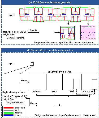
FIGURE 2 Dataset generation. (a) RGB diffusion model dataset generation and (b) Feature diffusion model dataset generation.
To discuss the influence of the condition tensor on model generation, this study examines three conditioning methods. The details are as follows.
Condition Type I: The input tensor consists of all tensors representing the drawings, whereas the condition tensor is derived by setting parts of the mask tensor to random numbers following a Gaussian distribution.
|
|
(1) |
Condition Type II: The input tensor consists of all tensors representing the drawings, whereas the condition tensor is derived by setting parts of the mask tensor to a fixed value of ��-1��.
|
|
(2) |
Condition Type III: The input tensor represents the shear wall layout, whereas the condition tensor comprises all the other tensors, excluding the shear wall layout.
|
|
(3) |
3.3 | Dataset description and data augmentation
The dataset used in this study is a supplementary version of the StructGAN dataset (Liao et al., 2022), encompassing 338 drawings. The dataset was divided into training, validation, and test datasets. To test the generalizability of the model, 18 drawings from design institutes that were distinct from those in the training dataset were included. The specific divisions of the training, validation, and test sets are listed in Table 3.
TABLE 3 Dataset split
|
Dataset name |
Length |
|
Train & validation (K-fold) |
320 |
|
Test A (the same design institute) |
18 |
|
Test B (different design institute) |
18 |
Considering the relatively small number of training samples in relation to the parameter size of the diffusion model, data augmentation methods were employed in this study to augment the training data volume. The data augmentation techniques utilized primarily encompassed horizontal flipping, vertical flipping, and translational transformations, aiming to preserve the features of the training samples. Through the application of these data augmentation techniques, a ��train & validation�� dataset comprising 62,720 (= 320 �� 4 �� 7 �� 7) images was obtained. The influence of data augmentation on the prediction results is discussed in Section 5.
4 | THE CONSTRUCTION, TRAINING, AND INFERENCE OF NEURAL NETWORK MODELS
To focus on the diffusion process features of the shear wall portion, this section introduces the construction, training, and inference methods for an image-prompt diffusion model with a mask tensor. The derivation of the diffusion model with a mask tensor is discussed in Section 4.1. The architecture and selection of the hyperparameters for the neural network are outlined in Section 4.2. Section 4.3 presents the training details of the diffusion model employed in this study.
4.1 | Derivation of image-prompt diffusion model with mask tensor
The diffusion model primarily comprises forward diffusion and reverse denoising processes. The forward diffusion process is a Markov process where Gaussian noise is added at each step (Ho et al., 2020):
|
|
(4) |
where ![]() are hyperparameters of the noise schedule. In this study,
the noise schedule is linear, which means that
are hyperparameters of the noise schedule. In this study,
the noise schedule is linear, which means that ![]() varies linearly from 0.000001 to 0.01 (Dhariwal et al., 2021).
When
varies linearly from 0.000001 to 0.01 (Dhariwal et al., 2021).
When ![]() , there is no distinction between
, there is no distinction between
![]() and Gaussian noise. It is noteworthy that Equation 5 can
be obtained:
and Gaussian noise. It is noteworthy that Equation 5 can
be obtained:
|
|
(5) |
where ![]() .
. ![]() actually measures the noise level, meaning that a smaller
actually measures the noise level, meaning that a smaller
![]() indicates that the image contains more noise. Ho et al. (2020)
presented a closed form of the posterior distribution of
indicates that the image contains more noise. Ho et al. (2020)
presented a closed form of the posterior distribution of ![]() given
given ![]() as
as
|
|
(6) |
Based on Ho et al. (2020), this study incorporated
a mask tensor. Given a noisy tensor ![]() ,
,
|
|
(7) |
The goal is to recover the target tensor
![]() . A neural network
. A neural network ![]() can be constructed, which takes condition tensor
can be constructed, which takes condition tensor ![]() , input tensor with noise
, input tensor with noise ![]() , and noise level
, and noise level ![]() as input and fits the noise vector
as input and fits the noise vector ![]() by optimizing the objective:
by optimizing the objective:
|
|
(8) |
Based on this, the
process of training the denoising diffusion model can be obtained, as outlined
in Table 4. For example, the input tensor
![]() , condition tensor
, condition tensor ![]() , and mask tensor
, and mask tensor ![]() can be sampled and a specific time step of
can be sampled and a specific time step of
![]() can be selected. The noise level
can be selected. The noise level
![]() can then be calculated. Subsequently, the noise
can then be calculated. Subsequently, the noise
![]() can be sampled from a Gaussian distribution
can be sampled from a Gaussian distribution
![]() . Equation 7 can be used to calculate the noisy input tensor
. Equation 7 can be used to calculate the noisy input tensor
![]() . The obtained tensor can be input to the neural network to
obtain the predicted noise generated by the neural network. By subtracting the
sampled true noise and utilizing the mask tensor as a mask, a loss value requiring
optimization can be obtained. Calculating the gradient of this loss value allows
the determination of the optimization direction for the neural network.
. The obtained tensor can be input to the neural network to
obtain the predicted noise generated by the neural network. By subtracting the
sampled true noise and utilizing the mask tensor as a mask, a loss value requiring
optimization can be obtained. Calculating the gradient of this loss value allows
the determination of the optimization direction for the neural network.
During the inference, based on Equation
7, an estimate of ![]() can be obtained as follows:
can be obtained as follows:
|
|
(9) |
By substituting Equation 9 into Equation
6, the estimated mean of the posterior distribution of ![]() given
given ![]() is
is
|
|
(10) |
Moreover, the variance of the posterior
distribution is set to ![]() (Ho et al., 2020). Based on this, the inference process can
be obtained as indicated in Table 4. First, Gaussian noise
(Ho et al., 2020). Based on this, the inference process can
be obtained as indicated in Table 4. First, Gaussian noise ![]() is sampled; then, based on this, the estimated input tensor
is sampled; then, based on this, the estimated input tensor
![]() at time step
at time step ![]() is calculated. Subsequently, the model is iterated continuously by
inputting the current time step��s
is calculated. Subsequently, the model is iterated continuously by
inputting the current time step��s ![]() and condition tensor
and condition tensor ![]() , with noise level
, with noise level ![]() to predict the noise tensor at the current time step. By
utilizing Equation 10, the predicted noise tensor enables the calculation of
the mean
to predict the noise tensor at the current time step. By
utilizing Equation 10, the predicted noise tensor enables the calculation of
the mean ![]() that represents the Gaussian distribution. With the computed
mean
that represents the Gaussian distribution. With the computed
mean ![]() and predetermined variance
and predetermined variance ![]() , sampling can be performed to obtain the previous time step��s
, sampling can be performed to obtain the previous time step��s
![]() , continuing this process until the predicted result
, continuing this process until the predicted result ![]() at the initial time step is obtained.
at the initial time step is obtained.
TABLE 4 Process of denoising diffusion model training and inference
|
Algorithm 1 Training |
|
|
1: |
repeat |
|
2: |
|
|
3: |
|
|
4: |
|
|
5: |
Take gradient descent step on |
|
|
|
|
6: |
until converged |

|
Algorithm 2 Inference |
|
|
1: |
|
|
2: |
|
|
3: |
for |
|
4: |
|
|
5: |
|
|
6: |
end for |
|
7: |
return |

4.2 | Neural network architecture and hyperparameters
The denoising model utilized in this study was a U-Net with an attention
mechanism and temporal encoding (Dhariwal et al., 2021). The U-Net architecture
displayed in Figure 3 was employed. The channel number of the input tensor with
noise ![]() , is denoted as N, where C represents
the channel number of the condition tensor
, is denoted as N, where C represents
the channel number of the condition tensor ![]() , and O represents the channel number
of the output tensor. The specific values of N, C, and O are listed in Table
5. For example, when utilizing the representation in feature space and Condition
Type ��, N is 6 (= 1 + 1 + 1 + 1 + 2), C is 6 (= 1 + 1 + 1 + 1 + 2), and O is
also 6 (N must equal O), based on Equation 1. H1, H2,
H3, and H4 represent the channel numbers of the intermediate
blocks in the U-Net. Specifically, the values of H1 and H2
are 64 and 128, respectively. H3 can be either 192 or 256; H4
can be 256 or 512 (Rombach et al., 2022). The appropriate parameters should
be chosen based on the model size; the influence of these parameters on the
model results is discussed in Section 5.2.
, and O represents the channel number
of the output tensor. The specific values of N, C, and O are listed in Table
5. For example, when utilizing the representation in feature space and Condition
Type ��, N is 6 (= 1 + 1 + 1 + 1 + 2), C is 6 (= 1 + 1 + 1 + 1 + 2), and O is
also 6 (N must equal O), based on Equation 1. H1, H2,
H3, and H4 represent the channel numbers of the intermediate
blocks in the U-Net. Specifically, the values of H1 and H2
are 64 and 128, respectively. H3 can be either 192 or 256; H4
can be 256 or 512 (Rombach et al., 2022). The appropriate parameters should
be chosen based on the model size; the influence of these parameters on the
model results is discussed in Section 5.2.
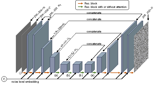
FIGURE 3 U-Net architecture.
TABLE 5 Values of N, C, and O obtained through different drawing representations
|
Space |
Condition Type |
N |
C |
O |
|
RGB |
- |
3 |
5 |
3 |
|
Feature |
�� |
6 |
6 |
6 |
|
Feature |
�� |
6 |
6 |
6 |
|
Feature |
�� |
1 |
5 |
1 |
It is important to note that the influence of the attention mechanism on the predictions is also discussed in this study. Owing to computational constraints, the addition of an attention layer is not feasible during downsampling by a factor of one or two because it would exceed the maximum allowable GPU memory capacity. Hence, the attention mechanism was primarily incorporated during downsampling by factors of four and eight. In Figure 3, the arrows labeled (a) and (b) indicate the potential positions for integrating the attention mechanism. The influence of attention positioning on predictions is discussed in Section 5.2.
4.3 | Training details
To investigate the influence of the aforementioned factors on the model results, 14 training sessions were conducted; the specific training numbers and corresponding model parameters are presented in Table 6. Among these:
(a) The ��ID�� column represents the ID name of the trained model. Models representing drawings in the RGB space start with the letter ��R��; those representing drawings in the feature space start with the letter ��F��. The subsequent numbers serve as labels. Trainings ending with ��-N�� indicate they were performed on datasets without data augmentation.
(b) ��Epoch�� represents the number of training loops. For example, Epoch 4199 denotes 4199 training loops.
(c) ��Seed�� denotes the selected random number seed. Random seeds govern different stochastic processes, such as the division of the training and validation sets, neural network weight initialization, and Gaussian noise sampling. If the random seeds are the same, they imply identical outcomes in these processes.
(d) For the explanation of ��C Type�� (Condition Type), please refer to Section 3.2.
(e) ��PRC�� indicates the precision with which the model is trained. For example, FP32 signifies training using true 32-bit floating numbers, whereas BF16 indicates training using bfloat16.
(f) For explanations regarding ��Att�� (Attention), ��H3��, and ��H4��, please refer to Section 4.2.
TABLE 6 Training details
|
Epoch |
Seed |
C |
PRC |
Att |
H3 |
H4 |
|
|
R1 |
4199 |
42 |
- |
FP32 |
No |
256 |
512 |
|
F1-N |
5299 |
42 |
�� |
FP32 |
No |
256 |
512 |
|
F1 |
7299 |
42 |
�� |
FP32 |
No |
256 |
512 |
|
F2 |
10399 |
88 |
�� |
FP32 |
No |
256 |
512 |
|
F3 |
10399 |
8888 |
�� |
FP32 |
No |
256 |
512 |
|
F4 |
13799 |
88 |
�� |
FP32 |
No |
256 |
512 |
|
F5 |
11199 |
88 |
�� |
FP32 |
No |
256 |
512 |
|
F6 |
17799 |
8888 |
�� |
FP32 |
(b) |
256 |
512 |
|
F7 |
22599 |
8888 |
�� |
FP32 |
(b) |
256 |
256 |
|
F8 |
13799 |
8888 |
�� |
BF16 |
(b) |
256 |
256 |
|
F9 |
18199 |
8888 |
�� |
BF16 |
(a & b) |
192 |
256 |
|
F10 |
12799 |
8888 |
�� |
BF16 |
(a & b) |
256 |
256 |
|
F11 |
23199 |
8888 |
�� |
BF16 |
(b) |
256 |
256 |
|
F12 |
15599 |
88 |
�� |
BF16 |
(b) |
256 |
256 |
It should be noted that the aforementioned training strategy remains consistent. That is, the model starts training with a learning rate of 5 �� 10-5 after tuning other hyperparameters. Mean Squared Error (MSE) is employed to compute the error in both the training and validation processes. Calculation of the validation error occurs every 100 epochs. Training ceases when the validation error demonstrates no decrease for 30 consecutive calculations. The model corresponding to the lowest validation error is selected for predictions and subsequent metric calculations. The ��Epoch�� in Table 6 indicates the total number of training loops undergone by the model. Furthermore, to ensure the reproducibility of the model, the random seed for the model is controlled as per the ��Seed�� provided in Table 6. This seed also governs the splitting method for the training and validation sets. When the seed value is the same, it can be inferred that the splitting method for the training and validation sets is identical. In addition, the average training time of the model on a single GPU is approximately 100 hours. The computing platform specifications were as follows: OS: Ubuntu 22.04 LTS; CPU: Intel Xeon E5-2682 v4 @ 64x 3GHz; RAM: 32 GB; GPU: NVIDIA GeForce RTX 3090 24 GB.
5 | DISCUSSION ON REPRESENTATION OF DRAWINGS, CONDITION TYPES, NEURAL NETWORK ARCHITECTURES, AND TRAINING HYPER-PARAMETERS
5.1 | Evaluation metrics
The Intersection over Union (IoU) metric (Equation 11) was primarily employed in this study for evaluation. It measures the morphological similarity between the design results of the diffusion model and ground truth by referencing StructGAN (Liao et al., 2021). The adoption of this metric is based on the research conducted by Liao et al. (2021), which suggests that structural design planning involves numerous implicit engineering experiences that are challenging to characterize succinctly in terms of quality. The design drawings used in this study were obtained from top-notch design institutes in China (Section 3.3), representing exemplary levels of engineering design. Hence, the similarity with engineers�� design outcomes (i.e., ground truth) is utilized to evaluate the AI design outcomes.
It is important to note that this IoU metric only considers the shear wall layout portion and is unrelated to the generation results of the other parts.
|
|
(11) |
where ![]() represents the tensor of the shear wall layout position predicted
by the diffusion model.
represents the tensor of the shear wall layout position predicted
by the diffusion model. ![]() is calculated using Equation 12.
is calculated using Equation 12.
|
|
(12) |
That is, the threshold for division is determined using the midpoint of the corresponding line between the wall and shear wall in space, i.e., the distances between the neural network output result and the points of the wall and shear wall in space are compared. If the result is similar to that of the shear wall, the output of the model is considered to represent the shear wall.
5.2 | Test results
The 14 models presented in Table 6 were tested using the ScoreIoU metric described in Section 5.1. Table 7 displays the prediction results of these 14 models on drawings from the same design institute as the training set (Test A). Each column in the table provides information on the model ID, validation loss, and the maximum, minimum, average, standard deviation, and median values of the ScoreIoU for the 18 drawing designs. Table 8 displays the prediction results of the 14 models on drawings from different design institutes compared to the training set (Test B). The results of the StructGAN and GNN model are included at the end of Table 8 to facilitate comparison of the relative performance of the Struct-Diffusion model. The appendix presents a selection of generated cases of Struct-Diffusion and StructGAN.
TABLE 7 Results of training cases on the Test A dataset
|
ID |
Valid Loss |
Max |
Min |
Mean |
Std |
Median |
|
R1 |
9.800 |
0.980 |
0.191 |
0.753 |
0.277 |
0.793 |
|
F1-N |
4.146 |
0.987 |
0.222 |
0.785 |
0.179 |
0.813 |
|
F1 |
4.018 |
0.987 |
0.476 |
0.799 |
0.155 |
0.830 |
|
F2 |
2.850 |
0.998 |
0.511 |
0.853 |
0.180 |
0.941 |
|
F3 |
2.967 |
0.998 |
0.360 |
0.807 |
0.187 |
0.857 |
|
F4 |
3.100 |
1.000 |
0.468 |
0.864 |
0.178 |
0.967* |
|
F5 |
8.681 |
1.000 |
0.604* |
0.873* |
0.151 |
0.960 |
|
F6 |
2.536* |
1.000 |
0.532 |
0.856 |
0.150* |
0.886 |
|
F7 |
2.903 |
1.000 |
0.191 |
0.811 |
0.212 |
0.878 |
|
F8 |
2.964 |
0.996 |
0.194 |
0.804 |
0.217 |
0.898 |
|
F9 |
3.060 |
1.000 |
0.348 |
0.804 |
0.188 |
0.866 |
|
F10 |
2.908 |
0.998 |
0.258 |
0.804 |
0.205 |
0.896 |
|
F11 |
8.534 |
1.000 |
0.222 |
0.813 |
0.199 |
0.886 |
|
F12 |
8.917 |
0.998 |
0.502 |
0.804 |
0.159 |
0.787 |
TABLE 8 Results of training cases on the Test B dataset
|
ID |
Max |
Min |
Mean |
Std |
Median |
|
R1 |
0.631 |
0.419 |
0.527 |
0.067 |
0.532 |
|
F1-N |
0.655 |
0.441 |
0.531 |
0.080 |
0.530 |
|
F1 |
0.694 |
0.475* |
0.552 |
0.056 |
0.540 |
|
F2 |
0.676 |
0.410 |
0.536 |
0.069 |
0.534 |
|
F3 |
0.664 |
0.426 |
0.544 |
0.060 |
0.543 |
|
F4 |
0.700* |
0.400 |
0.547 |
0.075 |
0.528 |
|
F5 |
0.659 |
0.459 |
0.552 |
0.058 |
0.545 |
|
F6 |
0.647 |
0.432 |
0.565 |
0.048* |
0.571 |
|
F7 |
0.694 |
0.469 |
0.585* |
0.062 |
0.579* |
|
F8 |
0.657 |
0.415 |
0.532 |
0.063 |
0.534 |
|
F9 |
0.658 |
0.345 |
0.550 |
0.064 |
0.549 |
|
F10 |
0.625 |
0.441 |
0.542 |
0.055 |
0.548 |
|
F11 |
0.698 |
0.336 |
0.542 |
0.080 |
0.561 |
|
F12 |
0.628 |
0.363 |
0.518 |
0.065 |
0.520 |
|
GAN |
0.505 |
0.224 |
0.363 |
0.073 |
0.368 |
|
GNN |
0.700 |
0.269 |
0.500 |
0.107 |
0.498 |
(1) Model Generalization Ability
When comparing the results of the same models in Tables 6 and 7, it can be observed that the ScoreIoU of Test B was consistently lower than that of Test A. This discrepancy arises from the design results of the training set originating from the same design institutes as the samples in Test A. In these drawings, the model could produce results similar to those of the designers. This indicates that the distribution of the test set was aligned with that of the training set, enabling the model to perform well on datasets with similar distributions. Notably, the ScoreIoU for all diffusion models in Test B exceeded 0.5, indicating reasonably similar images. This suggests that the model possesses certain generalization capabilities. To provide a more comprehensive assessment of the model��s inherent performance, subsequent comparisons primarily rely on the results of Test B. Specifically the Mean IoU presented in Table 7, unless stated otherwise.
(2) Influence of Drawing Representation Space
When comparing the models with IDs R1 and F1, the ScoreIoU of the F1 model was higher than that of the R1 model. This indicates that superior results can be achieved by utilizing the feature space to represent drawings. Furthermore, this finding confirms the accuracy of the analysis presented in Section 3.1. Consequently, the feature space was used to draw representations in the subsequent parts of this study.
(3) Influence of Data Augmentation
When comparing the models with IDs F1-N and F1, it was observed that the ScoreIoU of the F1 model was higher, despite having marginally longer training epochs and durations. This suggests that data augmentation can enhance the performance of the model, albeit at the expense of slower convergence. Given that the training phase was not significantly influenced by the training time, all subsequent training in this study employed datasets with data augmentation.
(4) Influence of Randomness
In practice, the partitioning of the training and validation sets, initialization of neural network weights, and sampling of Gaussian noise are all random processes, thus introducing certain randomness into the results of the model training. By comparing the models with IDs F1 and F2, models with IDs F3 and F4, and models with IDs F11 and F12, it can be deduced that if other conditions are held constant and only the random seed is changed, fluctuations will be observed in the final test results of the models. It should be noted that fluctuations caused by randomness did not influence the results of this study.
Furthermore, to minimize the influence of randomness on the conclusions of this section, the random seed was held constant when comparing the effects of different factors in this study.
(5) Influence of Condition Type
When comparing the models with IDs F2, F4, and F5, it is evident that the different condition types exert certain effects on the final output of the model. Condition Type III demonstrated the highest performance, followed by Condition Type II; Condition Type I was the least effective. Theoretically, when only the shear wall channel is output, the features of the model become denser, resulting in improved performance. However, considering the large number of parameters in the model, the differences in the final results between the three conditions were not significant. It should be noted that the validation loss results in Table 6 for Condition Type III are considerably higher than those for the other condition types. This discrepancy arises because of the generation of varying channel numbers and output formats, which render a direct comparison of the absolute values of the loss function meaningless.
(6) Influence of Attention Mechanism
The attention mechanism, by introducing the concept of weights, enables neural networks to focus more on local information (Vaswani et al., 2017). When comparing the models with IDs F3 and F6, it was observed that F6 incorporated an attention mechanism at the location depicted in Figure 3(b), resulting in a higher ScoreIoU. The attention mechanism enhances the ability of the model to extract global features by effectively enlarging the receptive field of the convolutional layer. Therefore, models with an added attention mechanism demonstrated clear superiority. Similarly, when comparing models with IDs F8 and F10, it was found that the F10 model included attention mechanisms at both locations, as indicated in Figure 3 (a) and (b) arrows, leading to a higher ScoreIoU. This suggests that incorporating attention when down-sampling by a factor of four positively influences the model. However, it is essential to note that the training and inference times for the F10 model were significantly longer than those for the F8 model. Thus, the trade-off between improved accuracy and decreased design efficiency must be carefully considered.
(7) Influence of Mixed Precision Training
Mixed-precision training, utilizing half-precision floating numbers, reduces memory consumption during gradient accumulation, thereby enhancing computational speed. Furthermore, the training outcomes achieved using mixed-precision training are comparable to those obtained using full precision (Micikevicius, 2017). When comparing the models with IDs F7 and F8, FP32 signifies training with a true 32-bit floating point, whereas BF16 represents training with bfloat16 mixed precision. It can be observed that the results of F8 are somewhat inferior to those of F7. However, the training time for F8 was significantly better than that for F7, and F8 also exhibited a more efficient GPU memory consumption than F7. Therefore, using BF16 as an alternative to FP32 is reasonable under specific circumstances. Training with FP16 can introduce substantial numerical instability, leading to training divergence. Hence, this study did not compare the results of FP16 training.
(8) Influence of H3 and H4
Another parameter that requires attention is the number of channels in the hidden layers. When comparing the models with IDs F6 and F7, it was observed that although H4 in F7 was only half that in F6, the results of F7 surpassed those of F6. Moreover, when comparing the models with IDs F9 and F10, the model with a smaller H3 achieved superior results. This was attributed to the relatively simple nature of the shear wall generation task in this study. Consequently, utilizing a model with more parameters has no meaningful significance and could even result in the model becoming trapped in local optima.
(9) Comparison with StructGAN and GNN
Based on the results presented in Table 8, the StructGAN model performed worse than the Struct-Diffusion model in terms of the ScoreIoU metric. The outputs generated by both StructGAN and Struct-Diffusion are displayed in Figure 4. The results obtained from StructGAN exhibit relatively blurry edges, whereas the outputs from Struct-Diffusion display clear and sharp boundaries. The performance of the GNN model lies between that of StructGAN and Struct-Diffusion. Compared to GNN, Struct-Diffusion exhibits a lower standard deviation in terms of ScoreIoU, indicating that its design results are more stable.

FIGURE 4 Comparison of outputs between StructGAN and Struct-Diffusion models. The red color represents the shear walls, the gray color represents the walls, and the green color represents the windows.
5.3 | Summary
This section examines the effects of different factors on the results of the diffusion model. In summary, the diffusion model tends to perform better when following the conditions outlined below.
(a) Regarding the dataset, it is recommended to represent drawings in the feature space, utilize Condition Type �� as the condition type, and apply data augmentation techniques.
(b) Regarding the model architecture, the addition of a suitable number of attention layers is recommended. The placement of these layers varies depending on the task performed. In addition, optimizing the number of channels in the hidden layers based on this problem is recommended.
(c) Regarding model training, the feasibility of employing a mixed-precision strategy should be considered. Although this approach could result in a decrease in model accuracy, it significantly improves the training efficiency.
Moreover, the proposed model not only performs well on the test set with the same distribution but also has better results on the test set with different distributions, with higher generalization capability compared to StructGAN. The model introduced in this study achieves higher quality and is more stable than the StructGAN and GNN methods.
6 | CASE STUDIES
In the previous section, the performance of Struct-Diffusion was analyzed from a metric perspective. In this section, case studies were conducted using selected typical examples from the Test A and Test B datasets to demonstrate the generative capabilities of the Struct-Diffusion model. The Struct-Diffusion model employed in this section was the model with ID F7, as listed in Table 6.
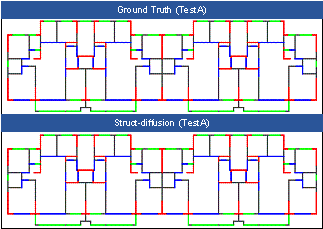
FIGURE 5 Comparison of structural designs of engineers and Struct-Diffusion (Test A dataset).
The results of the Struct-Diffusion model on Test A are displayed in Figure 5. The results generated by the model exhibit a high degree of similarity to the designs created by the engineer in terms of the ScoreIoU and inter-story drift ratio metrics, indicating its ability to effectively learn the design patterns employed by the same design institute and apply them to other cases.
For the selection of a typical example from the Test B dataset, a building located in Jiangsu Province, China, with a seismic design acceleration of 0.05 g (10% exceedance of 50 years), and height of 30 m was chosen. Both the Struct-Diffusion and StructGAN methods were utilized for the design; their respective design outcomes are depicted in Figures 6 and 7.
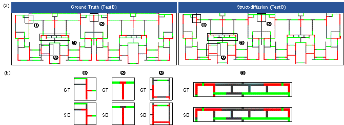
FIGURE 6 Comparison of structural designs of engineers and Struct-Diffusion (Test B dataset). (a) Global view and (b) Regional enlarged view.

FIGURE 7 Comparison of structural designs of engineers and StructGAN (Test B dataset).
Based on Figure 6(a), satisfactory performance was exhibited by the Struct-Diffusion model in this typical case. The general positions of the shear walls were accurately identified, with only minor discrepancies in certain details. Figure 6(b) illustrates the variation in the placement. The engineer��s design demonstrates more reasonable arrangements in areas �� and ��, whereas the arrangements in areas �� and �� necessitate judgment based on the actual circumstances. The aforementioned analysis highlights the commendable generalization capabilities of the Struct�Cdiffusion model, enabling it to perform effectively, even when addressing cases from diverse design institutes. Figure 7 displays the results generated by the StructGAN model for this building. Based on Figure 7(b), significant deviations from the engineering design are noticeable and the amount of shear wall placement significantly exceeds that of the engineering design, resulting in a less economical design.
Based on the seismic design intensity, structural height, and shear wall layout of a standard floor, mechanical analyses were conducted on the design results of a typical building (the same building as Figures 6 and 7) using a structural mechanics model (Lu et al., 2022). The inter-story deformation is essential to evaluate the structural performance under seismic loads (Lu et al., 2015; Lu et al., 2013). The results are displayed in Figure 8. It was observed that the results yielded by the Struct-Diffusion model closely aligned with the engineer's design, whereas the StructGAN design results deviated significantly from the engineer��s design. Moreover, as depicted in Figure 8, the inter-story drift ratio of the StructGAN design is notably smaller than that of the engineer��s design. This is attributed to the greater number of shear walls in the StructGAN model, resulting in greater rigidity and subsequent reduction in the inter-story drift ratio. Consequently, the StructGAN model is over-conservative, compromising its overall economic efficiency.

FIGURE 8 Comparison of inter-story drift ratio for different model designs. ��X�� is the direction of the strong axis, and ��Y�� is the direction of the weak axis.
7 | CONCLUSION
This study proposed an intelligent design method for shear wall structures based on a diffusion model. Through this method, the effective extraction of information from drawings and the arrangement of shear walls was achieved, surpassing the existing StructGAN method. The conclusions drawn from this study are as follows.
(a) A drawing representation suitable for diffusion models was proposed, and the influence of different condition types on the model results was discussed. Among these, the best performance was observed when the input tensor represents the shear wall layout, whereas the condition tensor comprises all the other tensors, excluding the shear wall layout.
(b) A mask tensor image-prompt diffusion model was introduced, and the corresponding training method for the diffusion model was derived. The ScoreIoU metric demonstrated the strong feature extraction capabilities of the proposed method, leading to a commendable performance in shear wall layout design tasks.
(c) The effects of the attention layer, hidden layer channel number, and mixed-precision training on the model architecture and training methods were discussed, resulting in a set of training strategies suitable for diffusion models.
(d) A comparison between the performance of the proposed Struct-Diffusion and StructGAN models was conducted, and the advantages and limitations of each model were analyzed using ScoreIoU and inter-story drift ratio (in elastic analysis) metrics.
The method proposed in this paper has been utilized to develop a corresponding API, which has been integrated into an intelligent design cloud platform (Qin et al., 2024). This API has been successfully applied to real-world intelligent design of shear wall structures, leading to a notable reduction in the design time for shear wall structures to a range of 5-10 minutes (Qin et al., 2024). According to the research by Fei et al. (2022), engineers typically require approximately 20 hours for shear wall layout design and 10 hours for modeling. This demonstrates the promising application prospects of this method.
It is important to note that the use of the diffusion model in this study remains in its preliminary stage. In addition, the model proposed in this study should be used mainly for preliminary design and is not a substitute for structural analysis. Currently, the diffusion model faces challenges such as unclear mechanical mechanisms and a lack of symmetry in design results. These issues require further research and improvements in subsequent studies.
The emergence of more powerful machine learning algorithms, such as the neural dynamic classification algorithm (Rafiei & Adeli, 2017) and the finite element machine for fast learning (Pereira et al., 2020), allows us to address the aforementioned issues using machine learning post-processing methods. Additionally, by training multiple sets of Struct-Diffusion models, following the dynamic ensemble learning algorithm (Alam et al., 2020), a more accurate and diverse placement of shear wall structures can be achieved.
Furthermore, due to the limited size of the dataset, the generalization performance of the current Struct-Diffusion model is still somewhat constrained. Future research can also consider leveraging self-supervised methods (Rafiei et al., 2024) to utilize unlabeled drawings for training, aiming to achieve better performance.
APPENDIX
This section presents a selection of generated cases of Struct-Diffusion and StructGAN.
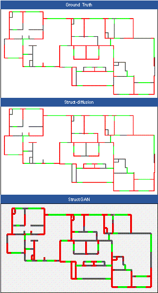
FIGURE A1 Comparison of designs across different models (Case 1)
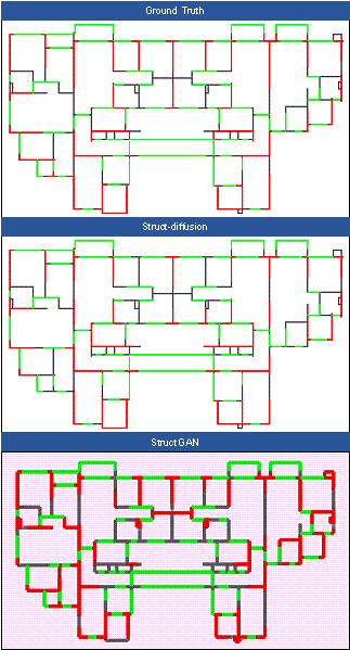
FIGURE A2 Comparison of designs across different models (Case 2)
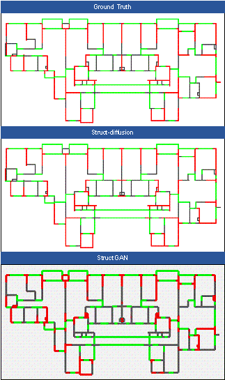
FIGURE A3 Comparison of designs across different models (Case 3)
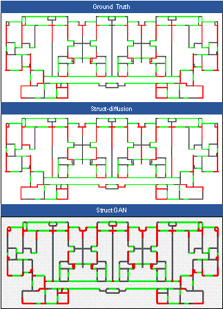
FIGURE A4 Comparison of designs across different models (Case 4)
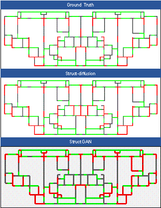
FIGURE A5 Comparison of designs across different models (Case 5)
ACKNOWLEDGMENT
REFERENCES
Adeli, H. (2001), Neural networks in civil engineering: 1989�C2000, Computer-Aided Civil and Infrastructure Engineering, 16(2), 126-142.
Adeli, H. (2020), Four decades of computing in civil engineering, in Ha-Minh, C., Dao, D. V., Benboudjema, F., Derrible, S., Huynh, D. V. K. & Tang, A. M. (eds.), Springer, pp. 3-11.
Alam, K. M., R., Siddique, N. & Adeli, H. (2020), A Dynamic Ensemble Learning Algorithm for Neural Networks, Neural Computing with Applications, 32(10), 8675-8690.
Batzolis, G., Stanczuk, J., Schönlieb, C.-B. & Etmann, C. (2021), Conditional image generation with score-based diffusion models. https://arxiv.org/abs/2111.13606
Boonstra, S., van der Blom, K., Hofmeyer, H. & Emmerich, M. T. M. (2020), Conceptual structural system layouts via design response grammars and evolutionary algorithms, Automation in Construction, 116, 103009.
Cao, H. Q., Tan, C., Gao, Z. Y., Xu, Y. L., Chen, G. Y., Heng, P.-A. & Li, S. Z. (2023), A survey on generative diffusion model. https://arxiv.org/abs/2209.02646
Chang, K.-H. & Cheng, C.-Y. (2020), Learning to simulate and design for structural engineering, International Conference on Machine Learning, PMLR, pp. 1426-1436.
CTBUH. (2020), Tall buildings in 2020: Covid-19 contributes to dip in year-on-year completions, CTBUH Research.
Danhaive, R. & Mueller, C. T. (2021), Design subspace learning: Structural design space exploration using performance-conditioned generative modeling, Automation in Construction, 127, 103664.
Dhariwal, P. & Nichol, A. (2021), Diffusion models beat GANs on image synthesis. https://arxiv.org/abs/2105.05233
Fei, Y. F., Liao, W. J., Huang, Y. L. & Lu, X. Z. (2022), Knowledge-enhanced generative adversarial networks for schematic design of framed tube structures, Automation in Construction, 144, 104619.
Fei, Y. F., Liao, W. J., Zhang, S., Yin, P. F., Han, B., Zhao, P. J., Chen, X. Y. & Lu, X. Z. (2022), Integrated schematic design method for shear wall structures: A practical application of generative adversarial networks, Buildings, 12(9), 1295.
Fu, B. C., Gao, Y. Q. & Wang, W. (2023), Dual generative adversarial networks for automated component layout design of steel frame-brace structures, Automation in Construction, 146, 104661.
Ho, J., Jain, A. & Abbeel, P. (2020), Denoising diffusion probabilistic models. https://arxiv.org/abs/2006.11239
Hofmeyer, H. & Delgado, J. M. D. (2015), Coevolutionary and genetic algorithm based building spatial and structural design, AI EDAM, 29(4), 351�C370.
Jenkins, W. M. (1998), Improving structural design by genetic search, Computer-Aided Civil and Infrastructure Engineering, 13(1), 5-11.
Kawar, B., Elad, M., Ermon, S. & Song, J. (2022), Denoising diffusion restoration models. http://arxiv.org/abs/2201.11793
Kicinger, R., Arciszewski, T. & De Jong, K. (2005), Parameterized versus generative representations in structural design: An empirical comparison, pp. 2007�C2014.
Liao, W. J., Huang, Y. L., Zheng, Z. & Lu, X. Z. (2022), Intelligent generative structural design method for shear wall building based on ��fused-text-image-to-image�� generative adversarial networks, Expert Systems with Applications, 210, 118530.
Liao, W. J., Lu, X. Z., Huang, Y. L., Zheng, Z. & Lin, Y. Q. (2021), Automated structural design of shear wall residential buildings using generative adversarial networks, Automation in Construction, 132, 103931.
Liu, H. H., Tian, Q., Yuan, Y., Liu, X. B., Mei, X. H., Kong, Q. Q., Wang, Y. P., Wang, W. W., Wang, Y. X. & Plumbley, M. D. (2023), Audioldm 2: Learning holistic audio generation with self-supervised pretraining. http://arxiv.org/abs/2308.05734
Lu, X. Z., Liao, W. J., Zhang, Y. & Huang, Y. L. (2022), Intelligent structural design of shear wall residence using physics-enhanced generative adversarial networks, Earthquake Engineering & Structural Dynamics, 51(7), 1657-1676.
Lu, X.Z., Xie, L.L., Guan, H., Huang, Y.L., & Lu, X. (2015), A shear wall element for nonlinear seismic analysis of super-tall buildings using OpenSees, Finite Elements in Analysis & Design, 98, 14-25.
Lu, X., Lu, X.Z., Guan, H., & Ye, L.P. (2013), Collapse simulation of reinforced concrete high-rise building induced by extreme earthquakes, Earthquake Engineering & Structural Dynamics, 42(5), 705-723.
Lugmayr, A., Danelljan, M., Romero, A., Yu, F., Timofte, R. & Van Gool, L. (2022), Repaint: Inpainting using denoising diffusion probabilistic models. http://arxiv.org/abs/2201.09865
Micikevicius, P., Narang, S., Alben, J., Diamos, G., Elsen, E., Garcia, D., Ginsburg, B., Houston, M., Kuchaiev, O., Venkatesh, G., Wu, H. (2017), Mixed Precision Training. https://arxiv.org/abs/1710.03740
Mirra, G. & Pugnale, A. (2021), Comparison between human-defined and ai-generated design spaces for the optimisation of shell structures, Structures, 34, 2950-2961.
Moehle, J. P. (2015). Seismic design of reinforced concrete buildings. New York: McGraw-Hill Education.
MOHURD. (2016). Code for the Seismic Design of Buildings (GB50011-2010). China Architecture & Building Press.
Nguyen, T.-H. & Oloufa, A. A. (2002), Spatial information: Classification and applications in building design, Computer-Aided Civil and Infrastructure Engineering, 17(4), 246-255.
Ning, M., Sangineto, E., Porrello, A., Calderara, S. & Cucchiara, R. (2023), Input perturbation reduces exposure bias in diffusion models. http://arxiv.org/abs/2301.11706
Pereira, D. R., Piteri, M. A., Souza, A. N., Papa, J. & Adeli, H. (2020), FEMa: A Finite Element Machine for Fast Learning, Neural Computing and Applications, 32(10), 6393-6404.
Qin, S. Z., Liao, W. J., Huang, S. N., Hu, K. G., Tan, Z., Gao, Y. & Lu, X. Z. (2024), AIstructure-Copilot: Assistant for generative AI-driven intelligent design of building structures, Smart Construction. https://elspub.com/papers/j/1745378442113941504
Rafiei, M. H. & Adeli, H. (2017), A New Neural Dynamic Classification Algorithm, IEEE Transactions on Neural Networks and Learning Systems, 28(12), pp. 3074-3083.
Rafiei, M. H., Gauthier, L., Adeli, H. & Takabi, D. (2024), Self-Supervised Learning for Electroencephalography, IEEE Transactions on Neural Networks and Learning Systems, 35(2), pp. 1457-1471.
Rodr��guez, J. d. M., Villafañe, M. E., Piškorec, L. & Caparrini, F. S. (2020), Generation of geometric interpolations of building types with deep variational autoencoders, Design Science, 6, e34.
Rombach, R., Blattmann, A., Lorenz, D., Esser, P. & Ommer, B. (2022), High-resolution image synthesis with latent diffusion models. http://arxiv.org/abs/2112.10752
Ruy, W.-S., Yang, Y.-S., Kim, G.-H. & Yeun, Y.-S. (2001), Topology design of truss structures in a multicriteria environment, Computer-Aided Civil and Infrastructure Engineering, 16(4), 246-258.
Saharia, C., Chan, W., Chang, H., Lee, C. A., Ho, J., Salimans, T., Fleet, D. J. & Norouzi, M. (2022), Palette: Image-to-image diffusion models. http://arxiv.org/abs/2111.05826
Sarma, K. C. & Adeli, H. (2001), Bilevel parallel genetic algorithms for optimization of large steel structures, Computer-Aided Civil and Infrastructure Engineering, 16(5), 295-304.
Savinov, N., Chung, J., Binkowski, M., Elsen, E. & Oord, A. v. d. (2022), Step-unrolled denoising autoencoders for text generation. http://arxiv.org/abs/2112.06749
Shahrouzi, M. & Pashaei, M. (2013), Tunnedttstochastic directional search: An efficient heuristic for structural optimization of building frames, Scientia Iranica, 20(4), 1124�C1132.
Sohl-Dickstein, J., Weiss, E., Maheswaranathan, N. & Ganguli, S. (2015), Deep unsupervised learning using nonequilibrium thermodynamics, International conference on machine learning, PMLR, pp. 2256-2265.
Song, Y., Sohl-Dickstein, J., Kingma, D. P., Kumar, A., Ermon, S. & Poole, B. (2020). Score-based generative modeling through stochastic differential equations. https://arxiv.org/abs/2011.13456
Tafraout, S., Bourahla, N., Bourahla, Y. & Mebarki, A. (2019), Automatic structural design of rc wall-slab buildings using a genetic algorithm with application in bim environment, Automation in Construction, 106, 102901.
Tashakori, A. & Adeli, H. (2002), Optimum design of cold-formed steel space structures using neural dynamics model, Journal of Constructional Steel Research, 58(12), 1545-1566.
Vaswani, A., Shazeer, N., Parmar, N., Uszkoreit, J., Jones, L., Gomez, A. N., Kaiser L. & Polosukhin I. (2017), Attention Is All You Need. http://arxiv.org/abs/1706.03762
Wang, L. F., Liu, J. P., Cheng, G. Z., Liu, E. & Chen, W. (2023), Constructing a personalized AI assistant for shear wall layout using stable diffusion. http://arxiv.org/abs/2305.10830
Zhao, P. J., Liao, W. J., Huang, Y. L. & Lu, X. Z. (2023a), Intelligent beam layout design for frame structure based on graph neural networks, Journal of Building Engineering, 63, 105499.
Zhao, P. J., Liao, W. J., Huang, Y. L. & Lu, X. Z. (2023b), Intelligent design of shear wall layout based on graph neural networks, Advanced Engineering Informatics, 55, 101886.
Zhao, P. J., Liao, W. J., Xue, H. J. & Lu, X. Z. (2022), Intelligent design method for beam and slab of shear wall structure based on deep learning, Journal of Building Engineering, 57, 104838.