1 Introduction

Expensive optimization problems (EOPs) are prevalent in the engineering domain, characterized by high computational costs required to derive the objective functions or constraints of optimization problems, such as conducting large-scale, detailed numerical simulations (He et al., 2023) . Evolutionary algorithms (EAs), widely applied to resolve EOPs, necessitate fitness evaluations of numerous candidate solutions during the search for an optimal solution, often incurring prohibitive costs (J.-Y. Li et al., 2022) . To address this issue, surrogate-assisted evolutionary algorithms (SAEAs) have been developed recently (G. Li & Zhang, 2021; Wei et al., 2021, 2023; Xie et al., 2023) . By employing surrogate models to substitute for detailed numerical simulations during the evolutionary optimization process, the SAEAs effectively reduce the costs of optimization (Y. Jin et al., 2019; Negrin et al., 2023) .

In the field of structural engineering, the optimization design of reinforced concrete (RC) shear-wall structures represents a classic EOP. Shear-wall structures, typically composed of shear walls, beams, and slabs, are extensively utilized in RC high-rise residential buildings in earthquake-prone areas. Engineers usually define several design variables based on actual situations, with each set of design variables corresponding to a candidate solution of the optimization problem and its associated fitness. During the schematic design phase of a shear-wall structure, engineers are tasked with finalizing design proposals within a matter of days. Within this period, structural engineers must complete all structural designs corresponding to multiple candidate architectural designs, and ensure that the structural designs meet physical and economic requirements through optimization, thereby placing stringent demands on the efficiency of the design optimization process.

In traditional optimization design of shear-wall structures, it is necessary to establish detailed physical models of each structural member within a chosen finite element software to analyze their physical responses under various working conditions such as gravity loads and earthquakes (Y. Li et al., 2011; X. Lu et al., 2013, 2015) . This is followed by conducting a detailed reinforcement design to ascertain material usage (Men et al., 2014) . For a typical shear-wall structure, this evaluation process can take approximately 5 min for a single candidate solution. Although EAs have proven to be highly effective in the optimization design of shear-wall structures (Gan et al., 2019; Zhou et al., 2022; F. Jin et al., 2023) , they often require hundreds of fitness evaluations to reach an acceptable local optimum. Consequently, the time taken for optimization design of shear-wall structures depends completely on detailed physical models; the use of EAs is prohibitively expensive and potentially impractical in circumstances such as the schematic design phase where a quick turnaround is desirable. To address the challenges mentioned above, SAEAs have been employed to reduce the optimization costs of RC shear-wall structures and other high-rise building structures. For instance, Lou et al. (2021) developed a data-driven tabu search algorithm that employed a support vector machine to evaluate the fitness of shear-wall structures. Huang et al. (2023) introduced a surrogate-assisted genetic algorithm that used a radial basis neural network during the optimization process to evaluate the natural periods of framed-tube structures. Similarly, Alanani & Elshaer (2023) presented an artificial neural network-assisted genetic algorithm for the layout design of shear walls in high-rise buildings. Z. Wang et al. (2023) proposed an optimization method based on surrogate model updating that utilized a generalized regression neural network to substitute for wind tunnel experiments and simulations during the design process of super-tall buildings.

Figure 1 Framework of traditional and proposed SAEAs

The typical framework and workflow of the SAEAs mentioned above, as presented in Figures 1(a) and 2, respectively, include four main parts: (1) Dataset establishment: Initialize and sample within the design space; perform numerical simulations on the samples to acquire evaluation results, which are then used as training samples. (2) Surrogate model training: Use design variables as inputs and the evaluation results as outputs; establish a machine-learning surrogate model based on the training samples. (3) Evolutionary optimization: Perform optimization based on evolutionary operators, employing either the surrogate model or a refined method for fitness evaluation. (4) Surrogate model updating: Add the design variables and the corresponding evaluation results by refined methods to the training samples, and retrain the surrogate model.

Note that, the input to the surrogate model (i.e., design variables) in part (2) is case-specific, meaning that the trained surrogate model only applies to that particular case during optimization. A new case necessitates re-execution of parts (1) and (2) to build a new dataset and train a new surrogate model. This limitation indicates that the existing SAEAs provide only a marginal increase in optimization efficiency compared to the EAs and may not fully meet the requirement of rapid optimization in the schematic design phase. For example, the SAEAs proposed by Lou et al. (2021) and Huang et al. (2023) have led to a saving in computational time by only 30% and 26%, respectively, compared to EAs without using surrogate models. Hence, there is an urgent need for an SAEA based on a generalizable surrogate model that, once trained, can be applied across a variety of structure cases (e.g., different shear-wall structures) without the need for retraining. This would significantly enhance the time efficiency of the existing SAEA, enabling it to meet the demands for fast optimization tasks during the schematic design phase.

The move towards a generalizable surrogate model indeed sets a higher bar for the model construction approach. Traditional machine learning methods used in current SAEA research efforts, such as Kriging, support vector machines, and artificial neural networks, are mostly designed to cater for specific cases (Negrin et al., 2023) . The limitations of these methods have been recognized for their typically single input form (vector) and the smaller number of trainable parameters, which hinders their ability to construct a generalizable representation suitable for laborious structural design tasks and to offer powerful nonlinear mapping capabilities required for predicting a diverse range of cases. Deep learning methods, which have risen to prominence recently, differ from traditional machine learning methods by allowing for diverse forms of input (such as images and graphs) and a large number of trainable parameters, rendering them wider applicability and better generalization capabilities. Graph neural networks (GNNs) represent a class of deep learning models based on graph representations, better suited for building structure design-related tasks (Chang & Cheng, 2020; Hayashi & Ohsaki, 2022; Zhao, Liao, et al., 2023) . The authors have laid a foundation for this study by proposing GNN-based surrogate models that can predict both physical responses and material usages of RC shear-wall structures (Fei et al., 2023, 2024) . After training on hundreds of shear-wall structures, these GNN surrogate models have shown promising generalizability to new structure cases. Despite these advances, the lengthy training time for GNN exceeds that of traditional machine learning models, making the conventional model updating approach of retraining (depicted in Figure 2) unsuitable. Therefore, this study is aimed at delving into how can GNNs be efficiently combined with EAs. A critical aspect of this study will be to find efficient ways to update the GNN without the necessity of retraining from scratch.

In response to the challenges mentioned above, this study presents a GNN-assisted EA that realizes rapid optimization design of shear-wall structures, with no need to rebuild the dataset and retrain the surrogate model when applied to new structure cases. The core innovations include the novel framework and workflow of GAEA, the generalizable GNN surrogate model, and the efficient updating strategy for the surrogate model. The rest of the paper is organized as follows: Section 2 introduces the framework of the proposed method and its data foundation. Section 3 formulates the shear-wall structure design task as an optimization problem. Section 4 introduces the GNN-based surrogate model. Section 5 proposes a distance-based surrogate model evaluation and updating strategy. Section 6 presents several typical case studies. Section 7 provides the major conclusions of this study.

2 Framework and dataset of GAEA

2.1 Framework

This study aims to propose a novel SAEA framework, referred to as the GNN-assisted evolutionary algorithm (GAEA). For a new case of a given structural system, such as a shear-wall structure, GAEA can establish a generalizable surrogate model in advance, which can be directly used for fitness evaluation without the need to reconstruct the dataset and retrain the surrogate model like traditional SAEAs.

The framework of the proposed GAEA is shown in Figure 1(b), and its workflow is presented in Figure 3. The proposed GAEA also consists of four parts: (1) Dataset establishment (Section 2.2): Collect hundreds of design cases of the targeted structural system, conduct detailed numerical simulations, obtain evaluation results, and use them as a dataset. (2) Surrogate model training (Section 4): Employ a universal representation method, using design information as input and evaluation results as output. Train a generalizable GNN-based surrogate model using the dataset. (3) Evolutionary optimization (Sections 3 & 5): Perform optimization based on evolutionary operators, convert design variables into design information, and perform fitness evaluations using the surrogate model or a refined method. (4) Surrogate model updating (Section 5): Multiply an error correction factor, which is chosen based on the distance between design variables, to the predictions of the surrogate model. The surrogate model is updated by adjusting the error correction factor, rather than retraining.

The major innovations and advantages of the proposed GAEA are: parts (1) and (2) can be completed in advance during leisure time prior to the optimization process. Once a design task is assigned and optimization is required to be completed in a timely manner, GAEA can employ the GNN-based surrogate model that has been pre-trained to accelerate the optimization design. In addition, when multiple structure cases are to be optimized, only parts (3) and (4) are required to be repeated. On the contrary, when using traditional SAEAs to optimize multiple cases, all four parts shown in Figure 2, including parts (1) and (2), must be repeatedly executed. Therefore, for practical engineering applications, the efficiency of GAEA is expected to be significantly higher than that of the traditional SAEAs.

Based on a survey of experienced structural engineers, the following three timing scenarios for optimization design can be well integrated with engineers' workflow during the schematic design phase:

(1) 10-minute optimization: Engineers can check optimization results after their 10-minute tea break.

(2) 45-minute optimization: 45 minutes is the longest time that engineers are willing to wait during their normal design pace.

(3) 120-minute optimization: Engineers can check the optimization results after their 120-minute lunch break.

In the following sections, the optimization design of RC shear-wall structures is taken as an example to verify the effectiveness of the proposed GAEA for the aforementioned three optimization timing scenarios.

2.2 Dataset for GNN training

To train a generalizable GNN surrogate model, it is necessary to collect as many design cases of the targeted structural system as possible. A total of 283 design drawings of RC shear-wall structures are collected from several renowned design institutes in China, from which the structural design and design conditions of the shear-wall structures are extracted. Structural design includes the layout and geometric dimensions of the shear walls and beams. Key design conditions consist of seismic, site, and height conditions, which are characterized by the design seismic acceleration ( ), site characteristic period ( ), and the number of stories ( ), respectively (Zhao, Fei, et al., 2023) . To enhance the diversity of the dataset and in turn improve the generalization capability of the GNN surrogate model, data augmentation is employed. Synthetic cases are generated by randomly changing the layout of the shear walls and beams or the design conditions based on real-world cases (Fei et al., 2024) . The dataset is expanded to four times its original size, resulting in a total of 1132 shear-wall structure cases.

For each shear-wall structure case in the dataset, parametric modeling is used to establish its finite element (FE) model for structural analysis and reinforcement design (Fei et al., 2022) , thereby obtaining the physical responses (inter-story drift ratio , torsional period ratio , shear-weight ratio , and axial compression ratio ) and material usages (concrete volume  and reinforcement mass ) required for fitness evaluation, as detailed in Section 3.2. Seventy or so cases that significantly deviate from the regulations of Chinese design codes are removed from the dataset, resulting in 1056 shear-wall structure cases.

Figure 4 Examples of the established shear-wall structure dataset

Finally, examples of the established dataset for shear-wall structures are presented in Figure 4. The input data are structural design and design conditions, while the label data (ground truth) are the physical responses and material usages. It should be noted that among these training data, some completely conform to the design codes, while others do not entirely comply; however, both types of data are crucial for the subsequent surrogate model training. This is because the structural designs at the early phases of optimization are often not code-conforming, while those at the later phases usually are. These two types of training data help the surrogate model to better adapt to the entire optimization process.

2.3 Typical cases for GAEA validation

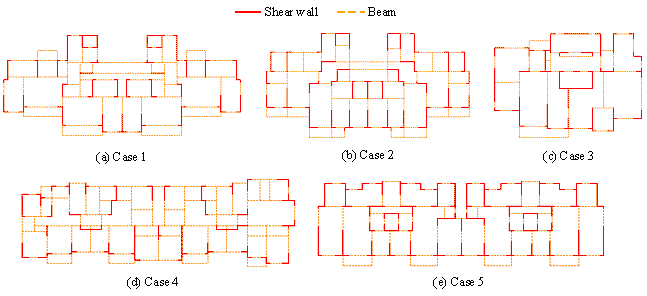
Figure 5 Initial structural layouts of typical shear-wall structures

Five typical shear-wall structure cases are selected for the GAEA validation. Their initial structural layouts (as shown in Figure 5) and design conditions (as presented in Table 1) are common and diversified. To verify the proposed GAEA, numerical experiments are carried out in Sections 4 & 5 based on the five shear-wall structure cases. The specific optimization results for three of the cases are provided in Section 6.

Table 1 Design conditions of typical shear-wall structures

Note:  is design seismic acceleration;  is site period;  is number of stories; C30, C35, C40, C45 stand for standard cubic compressive strengths of 30, 35, 40, 45 MPa, respectively; HRB400 stands for standard yield strength of 400 MPa.

3 Optimization problem of shear-wall structural design

The design of shear-wall structures is based on architectural design, and the layout of structural components must not affect the architectural space. The structural design includes three phases, namely schematic design, detailed design, and construction drawing design, with the first phase being the focus of this study. Specifically, in the schematic design phase, an initial design is typically carried out by experienced structural engineers or trained deep-learning models (Liao et al., 2021; Zhao et al., 2022; Feng et al., 2023) . Initial design usually includes the planar layout, section dimensions, and material grades of shear walls and beams, etc. Based on the initial design, optimization design is performed to adjust the shear-wall structure so that material cost is minimized while meeting the architectural requirements of the contractors and the physical requirements of the design codes. Since the shear-wall length is a core factor affecting the physical and economic performance of shear-wall structures (Zhou et al., 2022) , this study focuses on the optimization of shear-wall lengths.

3.1 Design variables

A typical shear-wall structure is shown in Figure 6. The planar layout of architectural components in the architectural design is shown in Figure 6(a), where the shear walls can only be placed within the location of the architectural walls. The planar layout of structural components in structural design is shown in Figure 6(b), which usually includes dozens of shear walls. To reduce the number of design variables, thereby simplifying the optimization complexity, connected shear walls are defined as shear wall groups, and the K-means algorithm is used to cluster these shear wall groups (Qin et al., 2024) . The clustering is based on features such as the shape and location of the shear wall groups, as detailed in Table 2. According to Qin et al. (2024) , the number of clusters is chosen as eight. Using increased numbers of clusters, e.g., 16 and 32, has been found to have a minor impact on the optimization results. After clustering the shear walls in Figure 6(b) into eight groups, the resulting clusters are shown in Figure 6(c).

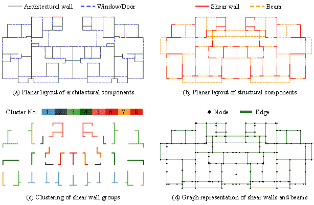
Figure 6 A typical shear-wall structure

Table 2 Features of shear wall groups for clustering (Qin et al., 2024)

Define a design variable vector , where the design variable  corresponds to the wall length of the i-th shear wall cluster. Here,  is a floating-point number, ranging from . The initial design corresponds to . When , all the wall lengths in the i-th shear wall cluster are considered to have reduced by 100%. When , all the wall lengths in the i-th shear wall cluster are regarded as having increased by 100%. When , all the wall lengths are altered proportionally in a similar manner. For common wall group shapes (T-shaped, L-shaped, C-shaped), the wall lengths corresponding to different design variable values are shown in Figure 7. In addition, the wall lengths are also subject to certain design rules: 1) the layout of shear walls shall not exceed the position of the architectural walls, to avoid affecting the building's functional space (as shown in Figure 6(a)); 2) according to the Chinese design codes, the ratio of the wall length to the wall thickness must not be less than 4 (MOHURD, 2010) .

When the shear wall lengths are changed, the beam lengths are adjusted accordingly without altering the topological relationship. The cross-sectional dimensions of the shear walls and beams are determined based on statistical rules (X. Lu et al., 2022; Zhao et al., 2022) . Note that the material grades are consistent with the initial design.

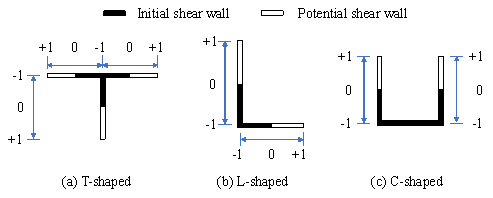
Figure 7 Relationship between design variable values and shear wall lengths

3.2 Objective functions

After comprehensively considering various factors in shear wall design and referencing existing related works (Men et al., 2014; Lou et al., 2021; Zhou et al., 2022; F. Jin et al., 2023; Qin et al., 2024) , this study adopts the following objective functions.

(1) Define an objective function  for the construction material quantity, which reflects the material cost of a shear-wall structure, as shown in Equation (1):

where  and  are the unit prices of concrete and steel reinforcement, respectively, determined according to the local market prices;  and  are the concrete volume and steel reinforcement mass of the structure, respectively.

(2) Define an objective function  for the inter-story drift ratio of the structure, which should not exceed the maximum limit specified by the design code, but also shall not be unnecessarily small, as expressed in Equation (2):

where  is the maximum inter-story drift ratio of the structure, and  is the maximum allowable inter-story drift ratio specified by the design code.

(3) Define an objective function  for the torsional period ratio of the structure, which should not exceed the maximum limit specified by the design code, and it shall be as small as possible, as shown in Equation (3):

where  is the torsional period ratio of the structure, and  is the maximum allowable torsional period ratio specified by the design code.

(4) Define an objective function  for the shear-weight ratio of the structure, which should not be smaller than the minimum limit specified by the design code, as shown in Equation (4):

where  is the minimum shear-weight ratio of the structure, and  is the minimum allowable shear-weight ratio specified by the design code.

(5) Define an objective function  for the axial compression ratio. This ratio should not exceed the maximum limit specified by the design code, as shown in Equation (5):

where  is the proportion of shear walls with an excessive axial compression ratio,  is the axial compression ratio of the i-th shear wall on the first story of the structure,  is the maximum allowable axial compression ratio of the i-th shear wall, and  is a function for counting the number of specified shear walls.

(6) Finally, define a total objective function  for transforming the multi-objective problem into a single objective problem, as shown in Equation (6) (Qin et al., 2024) , which is to be minimized.

Note that the maximum/minimum limits for physical responses are determined according to the local design codes (MOHURD, 2010) . In practical engineering projects, there is generally a safety redundancy in structural design. Therefore, the maximum or minimum limits specified by the design codes are increased or decreased by 10%, respectively, during the process of optimization.

Note also that the above definitions of the objective functions are only a feasible solution for the targeted design task. If the objective functions are defined for other tasks, the proposed GAEA can also be directly used to accelerate the optimization process. For example, some of the objective functions, e.g., , , , and , can be considered as constraint conditions, and a weighted sum can be used to transform the multi-objective problem into a single-objective one. The specific form of the objective functions and constraint conditions does not influence the effectiveness of the proposed GAEA, being a versatile optimization method.

In the optimization problem of this study, the fitness evaluation requires two material usage indicators (  and ) and four physical response indicators ( , , , ). For refined evaluations, the above-mentioned indicators can be obtained through parametric modeling and the FE models. For rapid evaluations, the above-mentioned indicators can be predicted using the GNN surrogate model described in Section 4.

4 GNN-based surrogate model

A generalizable surrogate model for the rapid optimization design of shear-wall structures must meet two key requirements. First, it must be able to comprehensively consider design information, especially the topological relationships between structural components, for accurate fitness evaluation. Second, once trained, it must be applicable to shear-wall structures of any scale, regardless of the number of structural components, so that a high evaluation efficiency can be ensured. Traditional machine learning methods cannot meet these requirements (as detailed discussed in Section 4.3), a GNN is therefore adopted in this study.

4.1 Graph neural networks

To evaluate the physical responses and material usages of shear-wall structures, it's necessary to consider the structural layout (topological information), component sizes (geometric information), and design conditions (textual information) simultaneously. To effectively integrate these heterogeneous input data, a GNN architecture recently proposed by the authors (Fei et al., 2023) , known as Graph-GEN, is used as the surrogate model. This method incorporates feature representation, feature aggregation, graph representation, and feature fusion algorithms specifically designed for tasks related to building structures, as depicted in Figure 8. Compared to traditional machine learning methods, Graph-GEN is a more generalizable surrogate model for the design of shear-wall structures.

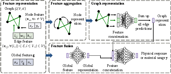
Figure 8 Architecture of Graph-GEN

Table 3 Input and output variables of Graph-GEN

To construct a surrogate model applicable to various shear-wall structure cases, a universal feature representation method is crucial. For any shear-wall structure, all its design information can be represented as a graph and a vector. Specifically:

(1) The structural design of the shear-wall structure is represented as a graph, which is compatible with the input format of GNNs. First, intersections of shear walls and beams are represented as nodes, and the shear walls and beams themselves are represented as edges. For example, the graph in Figure 6(d) is used to represent the structural layout in Figure 6(b). Additionally, planar coordinates of the intersections are used as node features (2-dimensional vector), and the geometric dimensions of the structural components (length, width, height) are used as edge features (3-dimensional vector), as presented in Table 3.

(2) The design conditions also significantly affect the physical responses and material usages of the shear-wall structure. Critical design conditions (design seismic acceleration , site characteristic period , and number of stories ) are represented as a global feature vector, as indicated in Table 3.

4.2 Surrogate modeling

According to the characteristics of various physical responses and material usages, the following approaches are adopted to construct their surrogate models:

(1) Several end-to-end data-driven surrogate models are established based on GNNs to predict the material usage (i.e., the concrete volume  and the steel reinforcement mass ), the first-order torsional period , and the story stiffness  (including flexural and shear stiffnesses in X and Y directions). Prior knowledge has been incorporated into the loss function or output layer of the GNNs to prevent the predicted material usage from falling below the minimum values required by design codes (Fei et al., 2023) and to avoid the prediction of negative values for physical quantities that should be positive (Fei et al., 2024) .

(2) The axial compression ratio  and the story mass  are directly calculated based on the design rules and physical principles.

(3) Based on the predicted story stiffness  and the calculated story mass , multi-degree-of-freedom flexural-shear models are established (Fei et al., 2024) . By conducting modal analyses on these multi-degree-of-freedom models, the first-order translational periods in the X and Y directions (  and ) can be obtained, which are then used to calculate the torsional period ratio . Further, by performing response spectrum analyses, the story displacements and shear forces under design-level earthquakes can be obtained, which in turn yield the inter-story drift ratio  and the shear-weight ratio .

(4) It should be highlighted that three strategies have been implemented to enhance the generalization performance of the surrogate models. First, a large-scale and diversified training set is collected, and its scale and diversity are further improved through data augmentation techniques. Second, general prior knowledge has been incorporated into the surrogate models to avoid making fundamental errors. Third, the surrogate models integrate data-driven and physics-based methods, making them less of a black box. Our previous works have also demonstrated that the surrogate models achieve high prediction accuracy on the test set, which is separate from the training set (Fei et al., 2023, 2024) .

It is important to note that when applying the surrogate model for fitness evaluation, the case-specific design variables should be transformed into the universal design information (graph and vector) before being fed into the surrogate model for model prediction.

4.3 Comparison with other machine learning methods

Due to its unique feature representation method and model architecture, the GNN being adopted in this study is considered superior to traditional machine learning methods in performing building structural design tasks.

For the feature representation method, the design information of building structures can be represented as a graph and a vector with complete topological, geometric, and textual information without missing any data. These graphs and vectors will be directly operated by the GNN, facilitating full capture of complex relationships in structural design tasks. In contrast, when using traditional machine learning methods, e.g., Kriging, support vector machine, or multilayer perceptrons, the design information of building structures can only be represented as a vector, which potentially causes a loss of the topological relationships of structural components.

For the model architecture, the GNN operations are iteratively performed on each node, its neighbors, and the connected edges. Therefore, the trained GNN model can be applied to graphs of any size, i.e., building structures with any number of structural components, featuring an excellent generalization capability. On the other hand, when using traditional machine learning methods, the trained model can only handle the input vector of a fixed size, resulting in poor generalization capability.

In the authors’ previous works (Fei et al., 2023, 2024) , the performances of the GNN and traditional machine learning methods (e.g., multilayer perceptrons) have been compared in detail. Our published experiment results indicate that the prediction accuracy of the GNN is significantly higher than traditional machine learning methods, thereby supporting the above statements.

Recently, novel machine learning techniques have garnered widespread attention in the fields of scientific computation and engineering simulation, with significant advancements including DeepONet (L. Lu et al., 2021) and physics-informed neural networks (PINNs) (Raissi et al., 2019; Cuomo et al., 2022) . These methods can be utilized to learn to solve physical problems, particularly those involving partial differential equations (PDEs). However, in the context of the optimization design of shear-wall structures, the key challenge lies in determining structural properties (e.g., story stiffness) and material usages based on design information. This determination is not controlled by PDEs but is instead based on calculation assumptions, construction requirements, empirical formulas, and other specifications as dictated by design codes. With the structural properties predicted, one can further employ well-established physical models (e.g., flexural-shear models) to carry out physical response calculations (typically matrix computation and eigenvalue analysis), swiftly obtaining the necessary responses without the need for machine learning predictions. Therefore, surrogate models such as DeepONet and PINNs, which are designed to solve physical problems, are not applicable to the optimization design tasks of shear-wall structures. On the contrary, the proposed GNN-based surrogate models are tailored for the intended design task and are, therefore, more suitable.

4.4 Prediction accuracy and efficiency

Numerical experiments are conducted on a personal computer equipped with an NVIDIA GeForce RTX 3090 GPU and an Intel Core i7-10700K CPU @ 3.80GHz. The Graph-GEN described in Section 4.1 is implemented based on the PyTorch deep learning framework (PyTorch, 2024) and trained on the GPU. The creation and operation of graphs are performed using the Deep Graph Library (DGL, 2024) . The modeling and optimization of shear-wall structures described in Section 3 are implemented through secondary development in commercial structural design software YJK-GAMA (GAMA, 2023b) , which provides robust toolboxes for parametric modeling, FE modeling, and EA, and is widely used in the Chinese construction industry.

Based on the dataset described in Section 2.2, the GNN surrogate models are trained and validated using the same method as reported in the previous works of the authors (Fei et al., 2023, 2024) . The hyperparameters of the GNN models are also selected based on our previous numerical experiments. The trained GNN surrogate models are used to predict the physical responses and material usages of the five typical cases described in Section 2.3. The objective functions are calculated according to the equations described in Section 3.2. The FE model evaluations by YJK-GAMA are used as the ground truth. The maximum and minimum percentage errors (PE) of the five cases and the mean absolute percentage error (MAPE) across the five cases are calculated. The results are presented in Table 4.

Table 4 Objective function errors of typical cases evaluated by GNN surrogate models

The results indicate that the MAPE of the total objective function is 7.4%, with the PE ranging from -5.2% to 16.9%. The MAPE for individual objective functions ranges from 1.1% to 8.0%, with the corresponding PE ranging from -17.8% to 17.6%. It is concluded that the GNN surrogate models are capable of performing an accurate fitness evaluation of shear-wall structures in most circumstances, but there are substantial errors in a few instances. Therefore, GAEA needs to employ the refined evaluation by the FE model to correct the rapid evaluation by the GNN surrogate models.

Within the environment of YJK-GAMA, a single fitness evaluation using the GNN surrogate models takes about 6 s, whereas using the FE model takes approximately 5 min. Hence, the evaluation efficiency of the GNN surrogate models is approximately 50 times that of the FE model.

5 Distance-based surrogate model evaluation and updating

5.1   Proposed strategy

For every new design variable vector generated during the optimization process, there are two different ways to conduct a fitness evaluation: (1) Rapid evaluation based on surrogate models: This involves quickly evaluating the design performance using GNN surrogate models, noting that surrogate models are an approximation of detailed numerical simulations and are inevitably prone to errors. (2) Refined evaluation based on FE models: This involves establishing a detailed FE model corresponding to the design variable vector to calculate its performance. The advantages and disadvantages of the refined evaluation are the exact opposite of rapid evaluation. The efficiency of refined evaluation is lower than that of rapid evaluation, but it has higher accuracy.

Combining the advantages of the above two methods, SAEA typically carries out both rapid and refined evaluations during the optimization process and uses the results of the refined evaluations to update the surrogate models, keeping the errors of rapid evaluations under control (Y. Jin et al., 2019) . Traditional SAEA uses conventional machine learning methods as surrogate models. The results of refined evaluations are used as new training samples, and the surrogate model can be updated by retraining the machine learning model. Since conventional machine learning methods have limited trainable parameters, their training generally takes only a few minutes or even seconds, making the cost of retraining acceptable. However, the generalizable surrogate model used in this study is based on a deep GNN (see Section 4), which has a large number of trainable parameters and requires hundreds of minutes to train. The cost of retraining the GNN is too high, thus necessitating a new strategy for model updating.

A distance-based surrogate model evaluation and updating strategy is proposed herein. The distances are measured between the design variable vectors of different candidate solutions. When the distances between different candidate solutions are small, an identical error correction factor can be used to adjust the predictions of the surrogate model. This avoids calculating the error correction factor for each candidate solution repeatedly, thereby saving computational time. The error correction factor is obtained by comparing the refined calculation results of FE models with the rapid prediction results of GNN.

The proposed method is feasible and applicable for optimization problems without high nonlinearity, e.g., shear-wall structural design in the schematic design phase, which requires only linear or equivalent linear analysis. In these circumstances, the following phenomena can be observed: The GNN model used in this study exhibits continuity, which forms the basis for using gradient-based algorithms (e.g., gradient descent) for training. Therefore, minor changes in the input to the model only result in slight variations in the model's predictions, as shown by the orange curve in Figure 9. Meanwhile, the ground truth that the model aims to predict is also continuous. Minor changes in the design information (e.g., the length of a shear wall) only cause small variations in the physical responses and material usage, as depicted by the blue curve in Figure 9. Hence, for minor changes in the model input, the error of the model prediction from the ground truth also varies marginally, as indicated by the shaded area in Figure 9. When the distances between several design variable vectors are small (e.g., x₁, x₂, and x₄ in Figure 9), the errors in their model predictions are relatively similar, and an identical error correction factor can be roughly used to adjust the evaluation results of the surrogate model. Definitions of distance and the error correction factor can be found in Section 5.2.

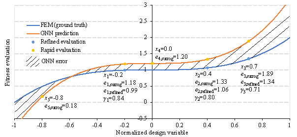
Figure 9 Schematic diagram of distance-based model evaluation and updating

Similar to the existing distance-based model updating methods (Branke & Schmidt, 2005) , the proposed method can enhance the exploration of unknown design spaces that have not been visited by the EA (Črepinšek et al., 2013) . However, existing distance-based model updating methods require adding refinedly evaluated design variable vectors to the training samples, followed by retraining of the surrogate model. In contrast, the proposed method does not require the surrogate model to be retrained but directly adjusts the prediction results, featuring a significant difference and advantage to the existing approaches.

5.2 Algorithm implementation

For a given design variable vector to be evaluated, calculate its distance d from the design variable vectors that have already been refinedly evaluated, to determine whether an identical error correction factor can be used. The definition of the distance d is given in Equation (7):

where  and  represent the design variable vector to be evaluated and the one that has been refinedly evaluated, respectively;  and  represent the i-th design variable of the vector to be evaluated and the one that has been refinedly evaluated, respectively; and n is the dimension or the number of design variables. The design variables should be normalized, i.e., , to ensure that the influence of each design variable on d is the same.

It can be observed that d is the Manhattan distance (Suwanda et al., 2020) between  and  divided by twice their dimension. The use of the Manhattan distance is due to its robustness being superior to the commonly used Euclidean distance, making it less susceptible to the influence of significant changes in individual design variables. After dividing by twice the dimension, the range of d becomes independent of the number of design variables, that is, . According to the requirements for optimization efficiency, a distance threshold  is defined.

(1) When the distance between two design variable vectors is small, that is, , the error correction factor of the refinedly evaluated vector can be used to adjust the vector to be evaluated, as shown in Equation (8):

where  is the adjusted evaluation result of the surrogate model for ,  is the original prediction result by the surrogate model for , and  is the error correction factor of the refinedly evaluated vector, as shown in Equation (9):

where  is the evaluation result of the refined method for ,  is the evaluation result of the surrogate model for .

Note that when multiple design variable vectors satisfy the distance threshold , Equations (8)-(9) should be calculated based on the refinedly evaluated design variable vector with the smallest distance.

(2) When the distance between two design variable vectors is greater than the predefined threshold , that is, , or there is no refinedly evaluated vector , the vector  should be refinedly evaluated based on FE model. Then, the refinedly evaluated design variable vector and its error correction factor should be recorded.

To facilitate understanding, Figure 9 provides a schematic diagram of a simple scenario, where there is only one design variable, i.e., n=1. Here, x₁, x₂, and x₃ are design variables that have been refinedly evaluated, while x₄ and x₅ are design variables awaiting evaluation. Define  and conduct a fitness evaluation for x₄ and x₅ outlined below.

(1) According to Equation (7), the distances from x₄ to x₁, x₂, and x₃ are 0.1, 0.2, and 0.35, respectively. Therefore, the distances from x₄ to both x₁ and x₂ are less than . x₁ is the closest to x₄, and the corresponding error correction factor γ₁=0.84, according to Equation (9). The adjusted evaluation result of x₄ is calculated as , according to Equation (8).

(2) According to Equation (7), the distances from x₅ to x₁, x₂, and x₃ are 0.3, 0.6, and 0.75, respectively. Therefore, the distances from x₅ to x₁, x₂, and x₃ are all greater than . In this situation, x₅ needs to be refinedly evaluated.

Algorithm 1 Surrogate model evaluation and updating strategy

Note:  is an empty set.

The details of the proposed surrogate model evaluation and updating strategy are elaborated in Algorithm 1. It is worth noting that the refinedly evaluated solutions are also used to update the surrogate model, as in traditional SAEAs. However, these solutions are not used to retrain the surrogate model. Instead, they are used to calculate an error correction factor. The surrogate model is updated by multiplying the prediction result by the error correction factor. The choice of the error correction factor depends on the distance between two solutions, as the term “distance-based” suggests.

5.3 Parameter assessment

Numerical experiments are conducted on the same personal computer as described in Section 4.4. The performance of the proposed GAEA is significantly influenced by the distance threshold , which determines the frequency of using FE models for refined evaluations. When , GAEA solely relies on FE models for refined evaluations and degrades into a traditional EA. When , GAEA exclusively uses the GNN surrogate model for rapid evaluations without updating the surrogate model. When , GAEA's fitness evaluations utilize both the FE model and the GNN surrogate model. This section will discuss the optimization outcomes and the time consumptions of GAEA for .

Meanwhile, the proposed strategy can be applied to both EA and SAEA to enhance their efficiency. The genetic algorithm (GA, a classic EA) and the online learning algorithm (OL, a widely used state-of-the-art SAEA) provided by YJK-GAMA (GAMA, 2023a) are used in this study as supporting algorithms. Online learning is an ensemble learning-based SAEA, utilizing several heterogeneous surrogate models for promoting ensemble diversity (Guo et al., 2019; Garza-Fabre et al., 2024) , such as polynomial regression, truncated Fourier series, support vector machine, and radial basis function networks.

For parameter selection, the number of fitness evaluations is chosen based on a parameter assessment. When the evaluation number is 50, the average reduction in the total objective function is 15.9%. When this number is 100, the average reduction is 22.1%, which is 6.2% lower than that from 50 evaluations. When this number is 200, the further reduction compared to 100 evaluations is smaller than 3%. Therefore, the number of fitness evaluations is set as 100, providing a balance between optimization time and effectiveness. The other parameters of GA and OL are set according to the recommendations in the YJK-GAMA official documentation, as given in Table 5. When employing different supporting algorithms and distance thresholds, different GAEAs are designated as shown in Table 6. To reduce the impact of case specificity on the experimental results, all experiments are repeated on the five typical cases presented in Section 2.3, and the results are averaged.

Table 5 Parameter setting of supporting evolutionary algorithms

Table 6 Details of different evolutionary algorithms

5.3.1 Comparison under identical numbers of fitness evaluations

When given an identical number of fitness evaluations (100 evaluations), the optimization outcomes are compared between the proposed GAEA and the traditional methods. After optimizations with various supporting algorithms and , the average reduction in the total objective function and the computational time are summarized in Table 7. Overall, the longer the computational time, the greater the reduction in the total objective function. The computational time in relation to the average reduction in the total objective function demonstrates a logarithmic relationship (R²=0.979). The effect of lengthening the computational time marginally decreases with the objective function getting smaller, as shown in Figure 10.

Table 7 Relative changes of the total objective function after optimizations

Experimental results demonstrate that for a fixed supporting algorithm, as  decreases, the objective function gradually declines while the time consumption gradually increases. This is due to the increased evaluation accuracy and time consumption of fitness evaluations as the frequency of FE model evaluations rises. As shown in Table 7, when , the percentage of refined evaluations is approximately 8%; when , this percentage increases to approximately 30%. Simultaneously, for a fixed , using OL as a supporting algorithm consumes more time but also yields better results. This is because OL requires training and updating of traditional machine-learning surrogate models, which consumes extra time compared to GA. However, by exploring the design space using the surrogate model, better design solutions can be discovered.

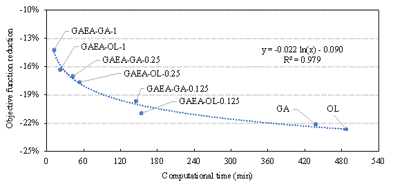
Figure 10 Relationship between average objective function reduction and computational time

On average, when , GAEA can achieve 64.4% of GA’s optimization outcome using only 2.8% of its computational time, or 72.1% of OL's optimization outcome using 4.5% of its computational time. When , GAEA can achieve 76.9% of GA's optimization outcome with 9.8% of its computational time, or 78.0% of OL's optimization outcome with 11.0% of its computational time. When , GAEA can achieve 88.9% of GA's optimization outcome with 33.2% of its computational time, or 92.5% of OL's optimization outcome with 31.6% of its computational time.

It is important to note that depending on the value of , GAEA can save 66.8% to 97.2% computational time compared to methods without employing GNNs. In contrast, other recently proposed SAEA methods only offer a reduction of computational time by 30% (Lou et al., 2021) and 26% (Huang et al., 2023) . Although the time reductions in this study are calculated based on different cases, they represent a fair comparison between the proposed GAEA and the existing SAEAs, without being influenced by the complexity of various cases. Therefore, the proposed GAEA has a significant efficiency advantage over the existing SAEAs.

5.3.2 Comparison under identical computational time

For a given identical computational time, the optimization outcomes are compared between the proposed GAEA and the conventional methods. As discussed in Section 2.1, the optimization time periods are set at 10, 45, and 120 min, respectively. These durations can well accommodate the working pace of engineers in the scheme design phase. According to the experimental results shown in Table 7, for a 10-min optimization task,  can be used; for a 45-min optimization task,  is suitable; and for a 120-min optimization task,  is recommended.

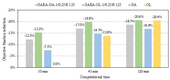
Figure 11 Objective function reduction for given identical computational time

Figure 11 shows the average reduction in the total objective function after being optimized by various algorithm configurations when the same computational time is consumed. It can be observed that the optimization outcome using OL as the supporting algorithm is superior to that when using GA. This is because OL itself constructs machine-learning surrogate models, which can search the design space more effectively. Therefore, it is recommended to use OL as the supporting algorithm of GAEA, and the following sections will compare the results of GAEA-OL with GA and OL. Specifically:

(1) When the available optimization time is 10 min, GAEA-OL-1 (-15.2%) > GAEA-GA-1 (-12.3%) > GA (-7.5%) >> OL (0.0%). This is because, within 10 min, GAEA can complete around 100 fitness evaluations through GNN. In contrast, GA can only perform several evaluations using FE models. OL, which needs to build a dataset, is yet to complete the training of the surrogate models within the 10-min time slot, and its optimization will not start. The total objective function reduction achieved by GAEA-OL-1 is significantly higher than the traditional methods, being 2.03 times that of GA.

(2) When the available time is 45 min, GAEA-OL-0.25 (-19.8%) > GAEA-GA-0.25 (-17.0%) > GA (-14.7%) > OL (-13.8%). At this point, OL has completed the training of the surrogate models, which significantly improves the efficiency of fitness evaluation, and its optimization outcome gradually approaches that of GA. Nevertheless, GAEA still maintains a leading advantage over GA and OL. The total objective function reduction achieved by GAEA-OL-0.25 is significantly higher than the traditional methods, being 1.43 times that of OL and 1.35 times that of GA.

(3) When the available time is 120 min, GAEA-OL-0.125 (-20.6%) > OL (-20.4%) > GAEA-GA-0.125 (-18.7%) > GA (-16.8%). This is because, as training samples related to this specific structure case are accumulated, the traditional case-specific surrogate model gradually approaches the generalizable GNN surrogate model in terms of evaluation accuracy. The total objective function reduction achieved by GAEA-OL-0.125 is slightly higher than the traditional SAEA, being 1.01 times that of OL. It is still significantly higher than the traditional EA, being 1.23 times that of GA.

Additionally, paired sample t-tests are conducted to evaluate the statistical significance of the mean reduction in the objective function by GAEA optimization compared to those by GA or OL. The null hypothesis states that the mean reduction in the objective function by GAEA optimization is less than that by GA or OL. The p-values for comparing GAEA-OL with GA and OL are presented in Table 8, and the significance level α is set as 0.1. A p-value lower than α leads to the rejection of the null hypothesis, suggesting that the mean reduction in the objective function by GAEA optimization is statistically not less than that by GA or OL. When comparing GAEA-OL-0.125 with OL, the null hypothesis cannot be rejected, indicating that GAEA-OL-0.125 is not significantly superior to OL. In other circumstances, the null hypothesis is rejected, affirming that the effectiveness of GAEA is statistically significant.

Table 8 P-values of the t-tests

To sum up, GAEA-OL-1/0.25/0.125 outperforms the traditional EA (i.e., GA) and a state-of-the-art ensemble learning-based SAEA (i.e., OL) for optimization timing of 10, 45, and 120 min, with a greater advantage at shorter optimization durations. When the optimization duration is long (e.g., 120 min), GAEA-OL-0.125 is not significantly superior to OL.

6         Case study

6.1 Detailed discussion on a typical case

To intuitively demonstrate the effectiveness of the proposed method for rapid optimization, a detailed case study is conducted on Case 5 of Section 2.3. The architectural design of Case 5 is illustrated in Figure 12(a), the clustering of the shear walls is shown in Figure 12(b), and the initial structural design is given in Figure 12(c). The design conditions are presented in Table 1. For the three optimization timing scenarios discussed in Section 2.1, the proposed GAEA (GAEA-OL-1/0.25/0.125, according to the recommendation given in Section 5.3.2), a traditional EA (GA), and a state-of-the-art ensemble learning-based SAEA (OL) are also used to perform the optimization design for Case 5. The parameter settings can be seen in Section 5.3.

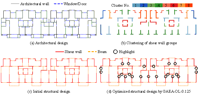
Figure 12 Design information and design result of Case 5

The physical responses and the material costs before and after optimization are shown in Table 9. As per the Chinese design code (MOHURD, 2010) , the shear-wall structure of Case 5 should meet the following criteria: , , and . Meanwhile, the material cost  and the proportion of shear walls with an excessive axial compression ratio  should be as small as possible. The initial structural design before optimization has an issue of having  exceeding the code limit. The results of the case study indicate that:

Table 9 Design performances of Case 5 before and after optimization

(1) After 10 min of optimization, the values of  resulting from the GA and OL’s designs still exceed the code limit, leading to a failed optimization, and  has not reduced significantly. All the physical responses of GAEA-OL-1’s design result comply with the design code, signifying successful optimization. However, its  increases by 1.3% compared to that of the initial design.

(2) After 45 min of optimization,  of the GA and OL’s design results again exceed the code limit, resulting in a failed optimization, although  has reduced significantly. All the physical responses of GAEA-OL-0.25’s design result comply with the design code, implying successful optimization. However, its  increases by 0.7% compared to that of the initial design.

(3) After 120 min of optimization, GA fails to find a better design scheme than the 45-min scenario, which is still a failed optimization. All the physical responses of GAEA-OL-0.125 and OL’s design results comply with the design code, confirming a successful optimization, and their  values are not increased compared to the initial design. The total objective function of GAEA-OL-0.125 is 3.7% lower than that of OL, resulting from its design result having a more rational safety redundancy. The structural design of GAEA-OL-0.125 after optimization is shown in Figure 12(d), and the differences between the optimized design from the initial one are highlighted with circles. It can be seen that the optimized structural design does not affect the functional space of the building and satisfies empirical design rules such as maintaining symmetry.

In summary, the proposed GAEA can meet the code compliance requirements of shear-wall structures for three optimization timing scenarios: 10, 45, and 120 min. Additionally, the longer the optimization duration, the better the design performance in terms of material cost and safety redundancy. Traditional GA fails to meet the rapid optimization needs for the aforementioned three scenarios, and existing OL fails for 10 and 45 min scenarios.

In engineering practice, the proposed GAEA can be easily integrated with the structural design software YJK-GAMA. Through secondary development, the FE model of the shear-wall structure will be updated in real-time in YJK-GAMA during the entire optimization process. After the optimization is completed, the FE model of the optimal design scheme can be seamlessly used in the subsequent phases for detailed design and construction drawing design. Therefore, a simple user training program will be sufficient for engineers to benefit from using the proposed GAEA.

6.2 Discussion on the scalability

To demonstrate the scalability of the proposed method on larger and more complex structures, two more case studies are conducted on Cases 1 and 2, which are high-rise buildings with 24 and 26 stories, respectively. For each case, 45 minutes are allocated for optimization design. The initial and the optimized structural designs are given in Figure 13, and the design metrics before and after optimization are given in Table 10 with highlighted values being discussed. As per the Chinese design code (MOHURD, 2010) , the shear-wall structure of Cases 1 and 2 should meet the same criteria as Case 5, except that  (Case 1) and  (Case 2).

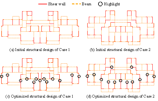
Figure 13 Design results of Cases 1 and 2

For Case 1, the initial structural design before optimization has issues of having  exceeding the code limit and having  that is too large. After 45 minutes of optimization, GAEA-OL-0.25’s design result has a  that complies with the code limit and a  that is 72.1% smaller. In contrast, GA and OL’s design results have a  that remains unchanged and a  that is only 47.1% and 36.7% smaller, respectively.

For Case 2, the initial structural design prior to optimization has issues of having  and  exceeding the code limit. After 45 minutes of optimization, GAEA-OL-0.25’s design result has both  and  complying with the code limit. In contrast, GA and OL’s design results still exceed the code limit, resulting in a failed optimization.

Therefore, the proposed GAEA demonstrates to have a good scalability and can be applied to the optimization design of high-rise buildings.

Table 10 Design performances of Cases1 and 2 before and after 45 minutes of optimization

7 Conclusions

This study proposes a GAEA for the rapid optimization design of RC shear-wall structures, highlighted by three key innovation tasks. First, a GAEA framework based on a generalizable surrogate model is proposed, which, unlike traditional SAEAs, does not require the reconstruction of datasets and retraining of surrogate models when encountering new structure cases. Second, a GNN surrogate model is proposed for evaluating physical responses and material usages, whose generalization performance is enhanced by augmenting the dataset, incorporating prior knowledge into the model, and integrating data-driven and physics-based methods. Third, a distance-based surrogate model evaluation and updating strategy is proposed, which can efficiently correct the prediction error of the GNN surrogate model without retraining, unlike the case of traditional SAEAs. Specific conclusions can be drawn as follows:

(1) The proposed GAEA framework is applicable to both traditional EA (e.g., GA) and traditional SAEA (e.g., OL). When different distance thresholds ( ) are set, GAEA can achieve 64.4% to 92.5% of GA or OL’s optimization outcomes with only 2.8% to 33.2% of their computational time. Compared to EAs without using a surrogate model, GAEA can save 66.8% to 97.2% of computational time, significantly surpassing the existing SAEA's 30% and 26%.

(2) During the time-critical schematic design phase, the optimization timing scenarios of 10, 45, and 120 min can accommodate the workflow of engineers, and GAEA achieves good optimization outcomes for all three time durations. When the available time is 10 min, the optimization by OL has not yet started, and the reduction in the total objective function by GAEA is 2.03 times that of GA. When the available time is 45 min, the reduction in the total objective function by GAEA is 1.43 times that of OL and 1.35 times that of GA. When the available time is 120 min, the reduction in the total objective function by GAEA is 1.01 times that of OL and 1.23 times that of GA.

(3) The case study indicates that the GAEA can meet the code compliance requirements of shear-wall structures within the specified optimization durations of 10, 45, and 120 min. Moreover, longer optimization durations correlate with better design performance in terms of material costs and safety redundancy. Traditional GA and OL, however, fail to fully meet the rapid optimization needs for the given time frames. Additionally, the GAEA demonstrates to have a good scalability and can be applied to the optimization design of high-rise buildings.

Despite the time efficiency and advantage of the proposed GAEA, some limitations are acknowledged herewith. Firstly, the GNN surrogate model cannot be directly adopted for column and brace designs in building structures, and the influence of the design loads has yet to be fully considered. Secondly, the proposed distance-based model updating strategy is not applicable for solving optimization problems with high nonlinearity, e.g., performance-based seismic design. Thirdly, it is difficult to further improve the prediction accuracy of the GNN surrogate models once their training process is completed.

To address the above limitations, the following roadmap can be followed in future research. The first step is to upgrade the feature representation method and model architecture of the GNN surrogate model so that all types of structural components and design loads can be considered. The second step is to explore other model updating strategies, such as fine-tuning the GNN with new training samples, for potential extension of the model to address highly nonlinear problems. The third step is to fully utilize the deep learning method in conjunction with optimization design. For example, the optimized cases can be added to the dataset and used in the retraining of the GNN, potentially further improving the GNN accuracy.

Acknowledgment

Data availability statement

The core of the proposed GAEA, i.e., a GNN-based surrogate model for predicting physical response and material usage, is deployed on an online server, and an application programming interface (API) is developed to facilitate its application. The API, the associated document, and relevant data for demonstration can be found in the GitHub repository (https://github.com/YifanFEI/GNN-assisted-EA).

References

Alanani, M., & Elshaer, A. (2023). ANN-based optimization framework for the design of wind load resisting system of tall buildings. Engineering Structures, 285, 116032. https://doi.org/10.1016/j.engstruct.2023.116032

Branke, J., & Schmidt, C. (2005). Faster convergence by means of fitness estimation. Soft Computing, 9(1), 13–20. https://doi.org/10.1007/s00500-003-0329-4

Chang, K.-H., & Cheng, C.-Y. (2020). Learning to simulate and design for structural engineering. Proceedings of the 37th International Conference on Machine Learning, 1426–1436. https://proceedings.mlr.press/v119/chang20a.html

Črepinšek, M., Liu, S.-H., & Mernik, M. (2013). Exploration and exploitation in evolutionary algorithms: a survey. ACM Computing Surveys, 45(3), 35:1-35:33. https://doi.org/10.1145/2480741.2480752

Cuomo, S., Di Cola, V. S., Giampaolo, F., Rozza, G., Raissi, M., & Piccialli, F. (2022). Scientific machine learning through physics–informed neural networks: where we are and what’s next. Journal of Scientific Computing, 92(3), 88. https://doi.org/10.1007/s10915-022-01939-z

DGL. (2024). Deep graph library tutorials and documentation. https://docs.dgl.ai/

Fei, Y., Liao, W., Lu, X. Z., & Guan, H. (2023). Knowledge-enhanced graph neural networks for construction material quantity estimation of reinforced concrete buildings. Computer-Aided Civil and Infrastructure Engineering, 39(4), 518-538. https://doi.org/10.1111/mice.13094

Fei, Y., Liao, W., Zhang, S., Yin, P., Han, B., Zhao, P., Chen, X., & Lu, X. Z. (2022). Integrated schematic design method for shear wall structures: a practical application of generative adversarial networks. Buildings, 12(9), Article 9. https://doi.org/10.3390/buildings12091295

Fei, Y., Liao, W., Zhao, P., Lu, X. Z., & Guan, H. (2024). Hybrid surrogate model combining physics and data for seismic drift estimation of shear-wall structures. Earthquake Engineering & Structural Dynamics, 53(10), 3093-3112. https://doi.org/10.1002/eqe.4151

Feng, Y., Fei, Y., Lin, Y., Liao, W., & Lu, X. Z. (2023). Intelligent generative design for shear wall cross-sectional size using rule-embedded generative adversarial network. Journal of Structural Engineering, 149(11), 04023161. https://doi.org/10.1061/JSENDH.STENG-12206

GAMA. (2023a). Faster finding of structural optimal solution: the use and characteristics of online learning algorithm. https://mp.weixin.qq.com/s/QAlskAsGKr4vGjOQAQv8pA (in Chinese)

GAMA. (2023b). YJK-GAMA secondary development guide. https://gitee.com/NonStructure/yjk-gama-secondary-development/ (in Chinese)

Gan, V. J. L., Wong, C. L., Tse, K. T., Cheng, J. C. P., Lo, I. M. C., & Chan, C. M. (2019). Parametric modelling and evolutionary optimization for cost-optimal and low-carbon design of high-rise reinforced concrete buildings. Advanced Engineering Informatics, 42, 100962. https://doi.org/10.1016/j.aei.2019.100962

Garza-Fabre, M., Cortés-García, N., Galeana-Zapién, H., & Landa, R. (2024). Surrogate models and ensemble strategies for expensive evolutionary optimization: an industrial case study. IEEE Access, 12, 86144–86159. https://doi.org/10.1109/ACCESS.2024.3416811

Guo, D., Jin, Y., Ding, J., & Chai, T. (2019). Heterogeneous ensemble-based infill criterion for evolutionary multiobjective optimization of expensive problems. IEEE Transactions on Cybernetics, 49(3), 1012–1025. https://doi.org/10.1109/TCYB.2018.2794503

Hayashi, K., & Ohsaki, M. (2022). Graph-based reinforcement learning for discrete cross-section optimization of planar steel frames. Advanced Engineering Informatics, 51, 101512. https://doi.org/10.1016/j.aei.2021.101512

He, C., Zhang, Y., Gong, D., & Ji, X. (2023). A review of surrogate-assisted evolutionary algorithms for expensive optimization problems. Expert Systems with Applications, 217, 119495. https://doi.org/10.1016/j.eswa.2022.119495

Huang, M.-F., Wang, C.-H., Lin, W., & Xiao, Z.-B. (2023). A multi-objective structural optimization method for serviceability design of tall buildings. The Structural Design of Tall and Special Buildings, 32(17), e2052. https://doi.org/10.1002/tal.2052

Jin, F., Yang, Y., Xiao, Z., Gao, B., & Lou, H. (2023). Shear wall layout optimization of multi-tower buildings based on conceptual design and extended evolutionary structural optimization method. Engineering Optimization, 56(4), 1–20. https://doi.org/10.1080/0305215X.2022.2161535

Jin, Y., Wang, H., Chugh, T., Guo, D., & Miettinen, K. (2019). Data-driven evolutionary optimization: an overview and case studies. IEEE Transactions on Evolutionary Computation, 23(3), 442–458. https://doi.org/10.1109/TEVC.2018.2869001

Li, G., & Zhang, Q. (2021). Multiple penalties and multiple local surrogates for expensive constrained optimization. IEEE Transactions on Evolutionary Computation, 25(4), 769–778. https://doi.org/10.1109/TEVC.2021.3066606

Li, J.-Y., Zhan, Z.-H., & Zhang, J. (2022). Evolutionary computation for expensive optimization: a survey. Machine Intelligence Research, 19(1), 3–23. https://doi.org/10.1007/s11633-022-1317-4

Li, Y., Lu, X. Z., Guan, H., & Ye, L. (2011). An improved tie force method for progressive collapse resistance design of reinforced concrete frame structures. Engineering Structures, 33(10), 2931–2942. https://doi.org/10.1016/j.engstruct.2011.06.017

Liao, W., Lu, X. Z., Huang, Y., Zheng, Z., & Lin, Y. (2021). Automated structural design of shear wall residential buildings using generative adversarial networks. Automation in Construction, 132, 103931. https://doi.org/10.1016/j.autcon.2021.103931

Lou, H., Gao, B., Jin, F., Wan, Y., & Wang, Y. (2021). Shear wall layout optimization strategy for high-rise buildings based on conceptual design and data-driven tabu search. Computers & Structures, 250, 106546. https://doi.org/10.1016/j.compstruc.2021.106546

Lu, L., Jin, P., Pang, G., Zhang, Z., & Karniadakis, G. E. (2021). Learning nonlinear operators via DeepONet based on the universal approximation theorem of operators. Nature Machine Intelligence, 3(3), 218–229. https://doi.org/10.1038/s42256-021-00302-5

Lu, X. Z., Liao, W., Zhang, Y., & Huang, Y. (2022). Intelligent structural design of shear wall residence using physics-enhanced generative adversarial networks. Earthquake Engineering & Structural Dynamics, 51(7), 1657–1676. https://doi.org/10.1002/eqe.3632

Lu, X., Lu, X. Z., Guan, H., & Ye, L. (2013). Collapse simulation of reinforced concrete high-rise building induced by extreme earthquakes. Earthquake Engineering & Structural Dynamics, 42(5), 705–723. https://doi.org/10.1002/eqe.2240

Lu, X. Z., Xie, L., Guan, H., Huang, Y., & Lu, X. (2015). A shear wall element for nonlinear seismic analysis of super-tall buildings using OpenSees. Finite Elements in Analysis and Design, 98, 14–25. https://doi.org/10.1016/j.finel.2015.01.006

Men, J., Shi, Q., & He, Z. (2014). Optimal design of tall residential building with RC shear wall and with rectangular layout. International Journal of High-Rise Buildings, 3(4), 285–296. https://doi.org/10.21022/IJHRB.2014.3.4.285

MOHURD. (2010). Technical specification for concrete structures of tall building (JGJ 3-2010). China Architecture & Building Press. (in Chinese)

Negrin, I., Kripka, M., & Yepes, V. (2023). Metamodel-assisted design optimization in the field of structural engineering: a literature review. Structures, 52, 609–631. https://doi.org/10.1016/j.istruc.2023.04.006

PyTorch. (2024). PyTorch documentation. https://pytorch.org/docs/stable/index.html

Qin, S., Guan, H., Liao, W., Gu, Y., Zheng, Z., Xue, H., & Lu, X. Z. (2024). Intelligent design and optimization system for shear wall structures based on large language models and generative artificial intelligence. Journal of Building Engineering. https://doi.org/10.1016/j.jobe.2024.109996

Raissi, M., Perdikaris, P., & Karniadakis, G. E. (2019). Physics-informed neural networks: a deep learning framework for solving forward and inverse problems involving nonlinear partial differential equations. Journal of Computational Physics, 378, 686–707. https://doi.org/10.1016/j.jcp.2018.10.045

Suwanda, R., Syahputra, Z., & Zamzami, E. M. (2020). Analysis of Euclidean distance and Manhattan distance in the K-means algorithm for variations number of centroid K. Journal of Physics: Conference Series, 1566(1), 012058. https://doi.org/10.1088/1742-6596/1566/1/012058

Wang, Z., Mulyanto, J. A., Zheng, C., & Wu, Y. (2023). Research on a surrogate model updating-based efficient multi-objective optimization framework for supertall buildings. Journal of Building Engineering, 72, 106702. https://doi.org/10.1016/j.jobe.2023.106702

Wei, F.-F., Chen, W.-N., Mao, W., Hu, X.-M., & Zhang, J. (2023). An efficient two-stage surrogate-assisted differential evolution for expensive inequality constrained optimization. IEEE Transactions on Systems, Man, and Cybernetics: Systems, 53(12), 7769–7782. https://doi.org/10.1109/TSMC.2023.3299434

Wei, F.-F., Chen, W.-N., Yang, Q., Deng, J., Luo, X.-N., Jin, H., & Zhang, J. (2021). A classifier-assisted level-based learning swarm optimizer for expensive optimization. IEEE Transactions on Evolutionary Computation, 25(2), 219–233. https://doi.org/10.1109/TEVC.2020.3017865

Xie, L., Li, G., Wang, Z., Cui, L., & Gong, M. (2023). Surrogate-assisted evolutionary algorithm with model and infill criterion auto-configuration. IEEE Transactions on Evolutionary Computation, 1–1. https://doi.org/10.1109/TEVC.2023.3291614

Zhao, P., Fei, Y., Huang, Y., Feng, Y., Liao, W., & Lu, X. Z. (2023). Design-condition-informed shear wall layout design based on graph neural networks. Advanced Engineering Informatics, 58, 102190. https://doi.org/10.1016/j.aei.2023.102190

Zhao, P., Liao, W., Huang, Y., & Lu, X. Z. (2023). Intelligent design of shear wall layout based on graph neural networks. Advanced Engineering Informatics, 55, 101886. https://doi.org/10.1016/j.aei.2023.101886

Zhao, P., Liao, W., Xue, H., & Lu, X. Z. (2022). Intelligent design method for beam and slab of shear wall structure based on deep learning. Journal of Building Engineering, 57, 104838. https://doi.org/10.1016/j.jobe.2022.104838

Zhou, X., Wang, L., Liu, J., Cheng, G., Chen, D., & Yu, P. (2022). Automated structural design of shear wall structures based on modified genetic algorithm and prior knowledge. Automation in Construction, 139, 104318. https://doi.org/10.1016/j.autcon.2022.104318