1. Introduction

Reinforced concrete (RC) frame structures are widely used in modern structural engineering, and the design of their sectional dimensions is important to ensure structural safety, cost-effectiveness, and environmental sustainability (Zhang et al., 2024). However, the traditional design process typically relies on the experience of structural engineers, leading to a high level of subjectivity and uncertainty in the design outcomes (Qin et al., 2025). The rapid development of artificial intelligence technology has led to new transformations in the field of engineering (Liang and Xue, 2023). In this context, generative models such as generative adversarial networks and diffusion models provide new possibilities for automated and intelligent structural design (Alcaide-Marzal and Diego-Mas, 2025; Liao et al., 2024).

Traditional intelligent design methods for frame structure component dimensions mainly involve various optimization methods. Heuristic algorithms such as genetic algorithms (Kaveh et al., 2013; Mariniello et al., 2022; Trapani et al., 2022; Xu and Gong, 2001), simulated annealing (Li et al., 2010), particle swarm optimization (Kaveh et al., 2020b), artificial bee colony algorithms (Kaveh et al., 2020a) , charged system search (Kaveh & Zakian, 2014) and enhanced colliding bodies optimization (Kaveh et al., 2016; Kaveh & Khavaninzadeh, 2023; Mottaghi et al., 2021), are widely used in the optimization of RC frame component dimensions (Kaveh, 2017; Kaveh, 2024). While proven effective in specific scenarios, these methods encounter significant challenges when applied to complex structural design problems (Peng et al., 2021). Heuristic algorithm-based optimization methods, in particular, are computationally intensive due to the involvement of large-scale design variables. For instance, the nonlinear finite element model (NFEM) utilized for the target structure necessitates iterative analyses for each combination of searched design variables during the optimization process, leading to high computational expenses (Qin et al., 2024). This issue is exacerbated when dealing with large-scale RC frame structures, where the multitude of design variables and intricate structural interactions can result in excessively long computation times.

The complexity of RC structures further compounds these challenges. The interactions between components and load effects, as well as the influence of seismic loads, vertical loads, and other external factors, introduce highly nonlinear and coupled features in the design space (Trapani et al., 2022; Xu et al., 2018). While NFEM modeling inherently accounts for these interactions and load effects, the iterative nature of heuristic algorithms still imposes a significant computational burden. For example, in structures with numerous beams and columns, each optimization iteration may require multiple NFEM analyses, potentially leading to computation times of several days or even weeks. This underscores a critical limitation of traditional heuristic algorithms, where efficiency significantly diminishes with an increase in the number of design variables.

Recent advancements have combined neural networks with surrogate models to speed up the optimization process (Kaveh et al., 1999; Zhang et al., 2024). However, these methods remain time-consuming, typically requiring 2 to 4 minutes, and are still prone to localized design issues due to the reliance on synthetic structural design datasets, which can make it difficult to capture the fundamental principles of project design. Given the demand for real-time design feedback and what you see is what you get capabilities, some researchers have turned to generative AI-based design approaches.

The emergence of models such as generative adversarial networks (GANs) and graph neural networks (GNNs) has introduced new methods for automated and efficient structural design. These algorithms, which learn from existing design drawings, can capture implicit knowledge of structural design. Compared with traditional optimization algorithms, they have demonstrated significant improvements in both computational efficiency and design rationality. Fu et al. (2023) proposed a method based on a Dual GAN for the layout design of steel frame structures, whereas Fei et al. (2022b), Liao et al. (2022, 2021), Lu et al. (2022), and Zhao et al. (2023) employed GAN methods for the intelligent design of shear wall structures. Fei et al. (2022a) utilized GAN methods for the intelligent design of framed tube structures. These methods leverage adversarial training with a large dataset, partially addressing the challenges of optimizing in highly nonlinear spaces and yielding promising results. In RC frame component design, it is necessary to predict the dimensions of the beams, slabs, and columns simultaneously. Because these components have significantly different features, GAN learning is not suitable, making it difficult for GAN-based design results to satisfy engineering requirements. Zhao et al. (2023) employed a GNN for shear wall layout design but did not address the component dimension design. Chang and Cheng (2020) integrated a GNN with genetic algorithms for frame structure dimension design; however, the limited fitting capability of the GNN to meet engineering demands led to less-than-ideal design results.

Recently, diffusion models have garnered attention as emerging generative models in many fields (Liu et al., 2023; Ning et al., 2023; Wei et al., 2025). Diffusion models operate by simulating data from high- to low-noise, in a reverse process, to gradually produce high-quality images (Ho et al., 2020). Compared with GANs, the diffusion model is a multistep generation method known for its higher generation quality and greater stability. It stands out in terms of conditional control and generating diversity (Saharia et al., 2022), making it a promising solution for intelligent structural design. Wang et al. (2023) and Zhou et al. (2024) utilized the Stable Diffusion weight fine-tuning method to consider design conditions such as story height and seismic design acceleration to generate layouts for shear walls. Gu et al. (2024) introduced a masked image-prompt diffusion model and developed a neural network called Struct-diffusion tailored for shear wall layouts, further improving the effectiveness of shear wall layout design. These studies primarily focused on shear wall layout design. To the best of the authors’ knowledge, no method is currently available for the design of dimensions of RC frame components based on the diffusion model.

In conclusion, the optimization of the design of dimensions of RC frame components encounters challenges stemming from the highly nonlinear behavior of traditional methods, fitting limitations of GNN, and sparse feature representation in GAN and diffusion models. Building on these identified challenges, this study investigated the utilization of a diffusion model in the dimension design of RC frame components. Through the integration of multichannel masks and gradient-weighted corrections, a design method that considers the features of the beam, slab, and column components was proposed. The contributions of this study are as follows.

a) A dimension design method for RC frame components based on the Diffusion Model was proposed, which enhanced the accuracy of the model by introducing multichannel masks and gradient-weighted corrections.

b) A dataset construction method suitable for the dimension design of RC frame components was developed, considering story-related features (e.g., story height) and building-related features (e.g., seismic design acceleration), and integrating multistandard story information for Diffusion Model learning.

c) The effectiveness of multichannel masks and gradient-weighted corrections in the dimension design of the RC frame components was validated. Through experimental comparisons and case studies, it was demonstrated that multichannel masks and gradient-weighted corrections significantly improved the model performance.

The remainder of this paper is organized as follows: Section 2 provides an overview of the overall methodology, Section 3 details the construction method of the dataset, Section 4 introduces the model architecture and its implementation details, Section 5 discusses the impact of various factors on the generated results of the Diffusion Model; Section 6 shows the generated results of typical cases. Finally, Section 7 presents the conclusions of this study.

2. Diffusion-based component dimension design method for RC frame structures

This study introduces a dimension prediction method for RC frame components based on a diffusion process called frame dimension diffusion. As illustrated in Figure 1, the proposed method consists of three main components: (a) dataset generation, (b) multimask diffusion model training, and (c) multimask diffusion model application.

(a) Dataset generation (Figure 1(a)): A novel representation method for RC frame structures is introduced to align the input and output requirements of the diffusion model. In this study, each layer of the RC frame structure is represented as an image, and each image contains multiple channels representing information on the component dimensions, layout, and design conditions. The dataset construction, incorporation of design conditions, and techniques for data augmentation, were extensively explored based on the proposed structural representation method as outlined in Section 3.

(b) Multimask diffusion model training (Figure 1(b)): Gu et al. (2024) introduced Struct-diffusion, a mask-based shear wall generation model, which improved the density of the data representation of the shear wall structure in the images. This study extends this concept by proposing a diffusion model that incorporates multichannel masks and gradient-weighted corrections. Input images with added noise are required by this model for noise prediction. The specific details of the input tensor and noisy tensor will be presented in Section 3.1. This model facilitates the simultaneous design of various component dimensions in a single prediction task by adjusting the weights to balance the representation densities of different component features within an image. This approach mitigates the problem of inadequate prediction performance for components with limited pixel proportions. The training process of the diffusion model is presented in Section 4, and the benefits of multichannel masks and gradient-weighted corrections are discussed in Section 5.

(c) Multimask diffusion model application (Figure 1(c)): Based on the training method outlined above, a dimension design model for RC frame components is obtained, enabling a more precise generation of RC frame component dimensions. The process of predicting the dimensions of the frame components using the model is shown in Figure 1(c). By leveraging this intelligent design approach, this study analyzes typical cases, as discussed in Section 6.

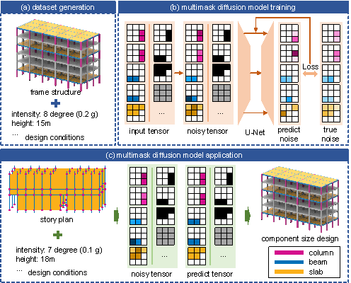
Figure 1 Diffusion-based design method for the component dimension of RC frame structures. (a) dataset generation, (b) multimask diffusion model training, and (c) multimask diffusion model application.

3. Dataset generation

The architectural design information of the frame structures can be conveniently processed into structured data (Chang and Cheng, 2020). The use of text-prompt methods may not provide direct guidance and may result in redundant information. Therefore, this study adopted an image-prompt method to guide the diffusion process (Gu et al., 2024). Moreover, the generation strategy of the Stable Diffusion method primarily focuses on producing a complete image (Rombach et al., 2022). However, in practice, the pixel count occupied by the frame columns and beams is considerably less than the total pixel count of the image ( , where N represents the number of pixels on the longer side of the image). Therefore, using the full-image generation approach directly would result in significant inefficiency and could introduce biases during neural network training. In addition, unlike the shear wall design task, in Struct-diffusion, there are notable variations in the number of pixels occupied by the beams, columns, and slabs. Therefore, a tailored multichannel mask method must be developed. Based on the above, this section delves into various dataset construction methods, along with the establishment of condition tensors, I/O tensors, mask tensors, and data augmentation strategies.

In this study, three distinct dataset construction methods are examined, each tailored to specific building characteristics, and these diverse construction approaches will be elucidated in Section 3.1. Moreover, this study suggests diverse strategies for incorporating design conditions to improve the performance of the diffusion model, as elaborated in Section 3.2. In addition, a range of data cleaning and augmentation strategies were applied to refine the dataset, boost the generalization capabilities of the model, and mitigate model instability. These are discussed in Section 3.3.

3.1 Methods of dataset construction

Figure 2 shows examples of the three dataset construction methods used in this study. For a single building, the consideration involves treating each actual story as a data point (Type A), each standard story as a data point (Type B), or the entire building as a data point (Type C). It is essential to highlight that Type C does not employ a strategy of linking each actual story; this decision is based on two considerations. First, the standard stories of an RC frame structure adequately capture the information of the structure, whereas the use of actual stories introduces substantial redundancy. Secondly, analysis of 133 sets of drawings reveals that RC frame structures typically comprise standard stories of up to 6 (≤6 standard stories constituting 99.25%), while some frame structures have actual stories surpassing 10 levels. Considering the memory constraints during model training, utilizing actual stories for connections is impractical. Therefore, Type C adopted the approach of connecting standard stories, as shown in Figure 2.

In Section 5, the influence of the Dataset Type on the efficacy of the RC frame component dimension design is examined.

Figure 2 Different types of dataset generation. Type A: considering each actual story as a single data point; Type B: considering each standard story as a single data point; Type C: considering each building as a single data point (linking all standard stories).

For each actual story, the method shown in Figure 3 was employed to encode the features in the feature space and alleviate the impact of erroneous priors on the model as recommended by Han et al. (2024). This study categorizes the features into two groups: story-related features (Figure 3 (a)) and building-related features (Figure 3 (b)). Story-related features, such as the dimensions of beams, columns, and slabs, arrangement of beams, columns, and slabs, loads on slabs, story heights, and story numbers, may vary across the different standard stories. However, building-related features, such as the total number of stories in the building, seismic design acceleration, characteristic period of the site, and frame seismic resistance grade, remained consistent within a given building.

This specific method involves transforming the current dimensions of the frame components into pixelated story plans. In this study, the image pixels were configured to 256 × 256 with a scaling ratio of 1 pixel = 300 mm between the image and drawings. The small dimensions of most components after scaling by this ratio are not conducive for AI training; therefore, all columns are denoted by 3 × 3 pixel rectangles, whereas the beams are denoted by 1-pixel-wide rectangles. Note that adjusting the scale ratio to 1 pixel = 300 mm scale ratio does not significantly affect this study, as it does not pertain to layout design. The key criterion is ensuring each component can be distinctly identified on the drawing.

After converting into pixelated story plans, dimension information is allocated to the component locations channel by channel, constructing the corresponding tensors. Figure 3(a) illustrates an example within a 3 × 3 pixel range. Here, column lx signifies the column width in the x-direction (measured in mm), whereas column ly denotes the column width in the y-direction (measured in mm). Notably, in this study, the x- and y-directions do not align with the strong and weak axes of the structure but rather with the local coordinate system of the columns. Nonrectangular columns, such as circular or pentagonal columns, are approximated as rectangular columns following engineering conventions. The interpretations of the beam height, beam width, and slab thickness tensors are self-evident. The column, beam, and slab masks indicate the positions of the columns, beams, and slabs, respectively, where a value of 1 signifies the presence of the corresponding component at that pixel point and 0 denotes its absence. The load tensor embodies the building loads with values sourced from the Load Code for the Design of Building Structures (MOHURD, 2012). Scalar values, such as the story height and story number in Figure 3(a), as well as the concrete material grade, total number of stories in the building, seismic design acceleration, characteristic period of the site, and frame seismic resistance grade in Figure 3(b), which are independent of the component positions, are directly expanded into 256 × 256 tensors. These tensors collectively constitute the feature tensors that delineate an RC frame structure.

Figure 3 Representation of RC frame structures. (a) feature of the stories, and (b) feature of the building.

3.2 I/O tensor, condition tensor, and mask tensor

To offer a more precise explanation of the inputs and outputs across various datasets, the notation from Struct-diffusion is adopted, focusing on the three tensors that are crucial to the model: the I/O tensor, condition tensor, and mask tensor. The I/O tensor represents the input and output tensors of the model. Following the derivation of the tensor representation of the feature space of the RC frame structure in Section 3.1, these representations are amalgamated into the I/O, condition, and mask tensors for the diffusion model. Given that the diffusion model requires a constant number of channels and that the maximum number of stories for all buildings in the dataset is six, this study establishes 6 as the standard number of stories for Dataset Type C. In cases where the standard number of stories falls below six, additional story-related data are padded with zeros. The rationale behind employing zero-padding is explained in Section 4.1. Table 1 lists the composition and respective number of channels for the I/O, condition, and mask tensors across different dataset types.

Table 1 I/O tensor, condition tensor, and mask tensor

Note: The component concrete grade includes the material grades of the columns, beams, and slabs, forming a three-channel tensor; the remaining tensors consist of a single channel.

3.3 Dataset cleaning and data augmentation

The dataset utilized in this study is an enhanced version of the dataset introduced by Qin et al. (2025). This study compiled a dataset from 133 RC frame structures from real-world engineering projects. The data originating from these projects were designed by well-established design institutes, ensuring high rationality and suitability for AI-driven design purposes. Initially, the dataset underwent data cleaning; the detailed cleaning methods and raw data distributions are available in Appendix A. The distribution of beam width and beam height post-cleaning is illustrated in Figure 4. For example, in Figure 4, the darkest color block represents that there are 3354 beams with a height of 500 mm and a width of 250 mm in the entire dataset. The distribution of column lengths in the x- and y-directions is presented in Figure 5, and the distribution of slab thickness is shown in Figure 6. Following the cleaning process, the beam dimensions are predominantly clustered in the central area, and the column lengths in both directions are primarily concentrated along the main diagonal, suggesting the prevalence of square or nearly square columns in this dataset. The majority of the slabs exhibit thicknesses of either 100 or 120 mm.

Figure 4 Distribution of beam width and beam height.
Note: Rows represent beam height, columns represent beam width, and the numbers inside the squares indicate the number of beams with the corresponding beam height and beam width values.

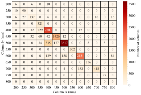
Figure 5 Distribution of column lx and column ly.
Note: Rows represent the column dimension in the y-direction, columns represent the column dimension in the x-direction, and the numbers inside the squares indicate the number of columns with the corresponding y- and x-direction dimensions.

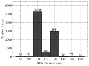
Figure 6 Distribution of slab thickness.

After data cleaning, the dataset comprises 109 buildings, with a total of 380 standard stories and 658 natural stories. The dataset is segmented into training, validation, and testing sets; the precise allocations are detailed in Table 2. To avoid data leakage, it was ensured that the natural stories of the test buildings in Datasets Types A and B were excluded from the training and validation sets.

Table 2 Dataset split

To address the limited number of training samples of the parameters in the diffusion model, data augmentation methods were also incorporated in this study to increase the amount of training data. The data augmentation techniques employed primarily encompass horizontal flipping, vertical flipping, and translation transformations to maintain the features of the training samples. By utilizing data augmentation techniques (Shorten and Khoshgoftaar, 2019), a training and validation dataset that is 196 times larger than the original dataset ( = 4 × 7 × 7) was generated. This is beneficial for training the diffusion model.

4. Architecture of the neural network model

Comparing the pixel categories in Figure 3, it is evident that the columns and beams occupy a minimal number of pixels in the overall image compared to the slabs. Specifically, in the image shown in Figure 3, the columns occupy only 432 pixels, the beams cover 1980 pixels, and the slabs encompass 17034 pixels. The ratio of the pixels taken up by the columns, beams, and slabs was approximately 1:4.58:39.43, which significantly influenced the learning efficacy of the neural network. To ensure that the diffusion process effectively captures information from the columns and beams, this section introduces multichannel mask and gradient-weighted correction image-prompt diffusion model construction, training, and inference methods. In Section 4.1, we primarily delve into the derivation of the multi-channel and gradient-weighted corrections, Section 4.2 will elaborate on the neural network architecture and hyperparameter selection, and Section 4.3 outlines the training specifics of the diffusion model in this study.

4.1 Derivation of the image-prompt diffusion model with multimask tensor and gradient-weighted correction

The diffusion model primarily consists of a forward diffusion process and a reverse denoising process. As Equation 1, the forward diffusion process is a Markov process where Gaussian noise is added at each step (Ho et al., 2020):

where  are hyperparameters of the noise schedule,  are input tensor in time t, t=0, 1, 2, 3, …, T, T is the time steps of the diffusion model,  means the conditional probability distribution of x given y,  means a multivariate normal distribution with a vector mean of  and a covariance matrix of . In this study, T=2000, and the noise schedule is linear, which means that  varied linearly from 0.000001 to 0.01 (Dhariwal and Nichol, 2021). When , there is no distinction between  and Gaussian noise. It is noteworthy that we can obtain the Equation 2:

where .  actually measures the noise level, meaning that a smaller  indicates that the image contains more noise. Ho et al. (2020) show a closed form of the posterier distribution of  given  as

Based on the work of Gu et al. (2024) and Ho et al. (2020), this study additionally incorporates a multi-mask tensor. Given a noisy tensor :

where  means beam height channel of noisy tensor .  means beam weight,  means column lx,  means column ly, and  means slab thickness,  means concatenate operator. We denote . The goal is to recover the target tensor , where  is the hadamard product operator. A neural network  can be constructed, which takes condition tensor , input tensor with noise and noise level  as input and fits the noise vector  by optimizing the objective

where , which is the gradient weighted correction item. Based on this, the process of training the denoising diffusion model can be obtained, as outlined in Table 3. The inference process is the same as Struct-diffusion.

Table 3 Process of denoising diffusion model training and inference

Notably, when  and , this method degenerates into the Struct-diffusion method. For Dataset Type C, we have the corresponding multimask tensors . Here, it is important to observe that if the corresponding standard story is empty, that is, as in the zero padding in Section 3.2, the objective function is a product of the Hadamard and mask, resulting in an outcome of 0. Hence, it was not considered during backpropagation. This enables compatibility with variable standard-story calculations.

In this study, we consider  as a single mask scenario, where  represent the layout of the beams, columns, and slabs obtained in Section 3.1. Setting  implies the absence of a gradient-weighted correction, whereas  signify the outcome when employing a gradient-weighted correction, where  denote the number of pixels occupied by beams, columns, and slabs in the image, respectively.

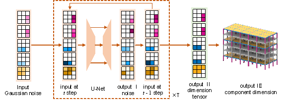
Figure 7 Relationship among the three outputs: Output I (noise prediction), Output II (tensor of component dimensions), and Output III (actual component dimensions).

In the discussion above, the neural network is primarily used for noise prediction, while the actual task in this study is to predict the component dimensions. In practice, there is a transformation required between these two stages. Figure 7 illustrates the three different outputs in this study and their relationships.

(a) Output I (noise prediction): This is the initial stage where the model learns to predict the noise added to the input images. This stage is essential for training the model and improving its ability to handle noisy input data.

(b) Output II (tensor output of component dimensions): This output is generated once the model has been trained, calculated based on T steps of Output I using the trained diffusion model.

(c) Output III (actual component dimensions): This output is derived from Output II by post-processing the tensor to extract the precise dimensions for the structural components.

4.2 Neural network architecture and hyper parameters

This study employed a U-Net with an attention mechanism and temporal encoding (Dhariwal and Nichol, 2021) as the denoising model. The U-Net architecture is illustrated in Figure 8, where N is the number of channels in the input tensor with noise , C is the number of channels in the condition tensor , and O is the number of channels in the output tensor. The specific values of N, C, and O are listed in Table 4. For instance, if Dataset Type A is utilized, based on Section 3.2, the number of channels in the input tensor with noise is 5, the number of channels in the condition tensor is 13, and the number of channels in the output tensor is 5 (the number of output tensor channels must be equal to the number of input tensor channels). H₁, H₂, H₃, and H₄ represent the numbers of channels in the intermediate blocks of U-Net. The values of H₁, H₂, H₃, and H₄ are 64, 128, 256, and 256, respectively (Gu et al., 2024). Moreover, the attention mechanism is incorporated during the 8× downsampling (Gu et al., 2024).

Table 4 Values of N, C, and O using dataset type

Figure 8 U-Net architecture

4.3 Training details

To investigate the impact of the various factors mentioned above on the model results, this study conducted seven sets of training sessions. The specific training IDs and corresponding model parameters are listed in Table 5. In this table, the ID columns represent the names of the trained models. The ID names are based on the dataset type, presence of multichannel masks, and weighted-gradient corrections. For example, for Dataset Type A with multichannel masks and no weighted-gradient correction, the model ID is A-MU. Here, “M” denotes Multimask, “S” denotes Single-mask, “U” denotes Unweighted, and “W” denotes Weighted. Notably, models with single-channel masks cannot undergo weighted-gradient correction because of the equal areas of the channel masks. Therefore, if a correction is applied, the weights corresponding to each channel will be the same, which is identical to no correction. The term epoch denotes the number of training cycles, and Epoch 21600 signifies a total of 21600 training cycles. Seed indicates the chosen random seed, which controls processes such as neural network weight initialization and Gaussian noise sampling. If the random seeds are the same, identical outcomes are obtained for these processes. Importantly, each training set has three random seeds, indicating that each set undergoes three training runs to reduce the impact of random errors on the conclusions of this study. The Training hours column represents the total training time. Further explanations of Dataset Type can be found in Section 3.1, and detailed descriptions of the mask type and weighting are provided in Section 4.1.

Table 5 Training details

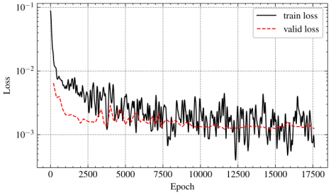
Figure 9 Loss curve

The training strategy for the aforementioned experiments was consistently maintained. The models were trained with a learning rate of 5 × 10^-5 following the optimization of other hyperparameters (Ho et al., 2018). Mean square error calculation was employed for the training and validation processes. Validation error assessment occurred every 200 Epochs, and training concluded after 30 consecutive validations without enhancement. Figure 9 gives a typical loss curve for diffusion model training. As shown in Figure 9, training is stopped when the validation loss does not decrease for 6000 (=200 × 30) epochs. At this point, the model has not overfitted to the training dataset. Additionally, the validation loss is close to the training loss, indicating that the model has a certain level of generalization ability. The model with the minimal validation error was chosen for prediction and subsequent metric computations. Furthermore, to ensure model reproducibility, the random seed specified in Table 5 governed the random initialization of the model, irrespective of the dataset splitting methodology. To ensure equitable comparisons, the dataset-splitting method remained uniform. Table 5 also presents the training duration of the models (in hours, on a single GPU). The computing platform configuration included OS: Ubuntu 22.04 LTS; CPU: Intel Xeon E5-2682 v4 @ 64x 3 GHz; RAM: 32 GB; GPU: NVIDIA GeForce RTX 3090 24 GB.

5. Discussion on dataset type, mask type, and gradient weighted correction

5.1 Evaluation metrics and postprocessing

Following the methodology proposed by Qin et al. (2025), this study employed the Root Mean Square Error (RMSE) metric for evaluation. This metric calculates the root mean square error between the results obtained from the diffusion model design and the engineering design (Ground Truth, GT). This metric was chosen because it maintains the same units as the original data, allowing for a direct assessment of the variability in the corresponding predicted results. In this study, we compared the RMSE values for the beam height, beam width, and column length in the x-direction, column length in the y-direction, and slab thickness. Notably, in practical design, the modulus is often applied. For example, if the designed beam width is 195 mm, it can be rounded up to 200 mm. Typically, the modulus for the beams and columns is 50 mm, whereas that for the slabs is 20 mm.

For the predictions produced by the diffusion model, the average values of the respective channels for each component were extracted to obtain the dimensional details of that component. Subsequently, by consolidating all dimensional information of the building, the RMSE was computed as an evaluation metric. Hence, the RMSE is component-centric rather than pixel-centric and is aligned with real-world applications.

5.2 Test results

Using the RMSE metric provided in Section 5.1, the seven sets of models listed in Table 5 were tested, and Table 6 presents the average performance of these models on the prediction dataset. Each column in the table represents the model ID as well as the RMSE values for the beam width, beam height, and column length in the x-direction, the column length in the y-direction, and slab thickness, all measured in millimeters. Additionally, Table 6 includes the results of the HetGNN model (Qin et al., 2025) for comparison, with the aim of evaluating the performance of the frame-dimension-diffusion model against the GNN methods.

Table 6 RMSE for the Test dataset (unit: mm)

(1) Dataset Type

Upon comparing the results for IDs A-MW, B-MW, and C-MW, it is evident that the prediction results for Dataset Types A and B are similar, while Dataset Type C significantly outperforms the other two. This can be attributed to Dataset Type C being obtained by considering the interconnections between different standard stories of a building, whereas Dataset Type A and B being obtained by treating different stories as distinct data points. Furthermore, it was observed that the Type C dataset showed a more pronounced improvement in the prediction of the vertical components, such as columns. This is because the vertical components must account for upper-story loads, making accurate predictions more challenging in the absence of upper-story information.

(2) Mask Type

By comparing the results of IDs A-S with A-MU or B-S with B-MU, it can be observed that the multichannel masks outperform the single-channel masks. In the case of the column and beam channels, the absence of multichannel masks leads to a high number of zero values, significantly surpassing the valid values. This scenario can mislead the neural network during backpropagation because it may predict the positions directly as zeros, thereby causing larger prediction errors. Additionally, it is noticeable that the improvement in prediction errors for slabs is relatively minor compared to that for beams and columns, which aligns with the aforementioned discussion.

(3) Gradient Weighted Correction

Comparing the results for IDs A-MU with A-MW or B-MU with B-MW, it is evident that after the weighted gradient correction, there is a noticeable decrease in the prediction errors related to the beam and column dimensions, whereas there is a slight increase in the prediction error for the slab thickness. Owing to the larger number of pixels occupied by slabs compared with that by beams and columns, the model without weighting is more likely to learn the prediction of slab thickness. However, the weighted model can better balance the prediction results for beams, columns, and slabs. Additionally, it is important to note that different normalization parameters were used for different channels, resulting in relatively large RMSE values between the different components and dimensions, as listed in Table 6. Table 7 presents the normalized RMSE results for the Dataset Type B models, representing the RMSE of the actual output of the diffusion model. The B-MU model shows a significant difference in predicting the slab thickness compared with its prediction of the beam and column dimensions. By contrast, the B-MW model does not exhibit this phenomenon, indicating that the weighted model can achieve a more balanced prediction error for the beams, columns, and slabs.

Table 7 RMSE for the Test dataset (normalized)

(4) Comparison with HetGNN

This study compared the Frame-dimension-diffusion model with the HetGNN model (Qin et al., 2025), which employs heterogeneous graph neural networks for predicting the dimensions of RC frames. Notably, except for beam width prediction, the prediction errors for other structural components were smaller in comparison to those obtained using HetGNN. Moreover, the variance in the prediction error for beam width between the C-MW and HetGNN methods was minimal, mostly falling within the error range demonstrated by the neural network models. This suggests that the Frame-dimension-diffusion approach holds a certain advantage in forecasting the dimensions of RC frame components.

5.3 Summary

This section analyzes the impacts of various factors on the results generated by the diffusion model. The model utilizing Dataset Type C, multichannel masks, and gradient-weighted correction achieved the best performance. Furthermore, the top-performing model had all the dimensional predictions within one modulus, except for the beam-height prediction, which was within two moduli. It can be concluded that this method is suitable for predicting the dimensions of the RC frame components.

6. Case studies

In Section 5, the performance of the Frame-dimension-diffusion model was evaluated based on the metrics. This section presents a case study using typical instances from a test dataset to demonstrate the generative capabilities of the Frame-dimension-diffusion model. The model utilized is identified as C-MW, as indicated in Table 5.

The case study presented in Section 6 focuses on a typical 6-story RC frame structure located in Hunan Province, China. This structure is a primary school dormitory with a story height of 3.5 m, a total building height of 21.15 m, a seismic design acceleration value of 0.10 g, a site characteristic period of 0.35 s, and first-grade frame seismic resistance. The beams, slabs, and columns are composed of C30 concrete. The structure consists of two standard stories, representing Stories 1 to 5 and the 6^th story. The Frame-dimension-diffusion model was used in the design. Subsequently, the YJK analysis software was used to analyze the inter-story drift ratio and construction material quantity (Qin et al., 2025) and compared it with the results from the engineering design. Table 8 compares the results from HetGNN and Frame-dimension-diffusion. It is evident that, in this instance, the RMSE of the Frame-dimension-diffusion output is within one modulus. Meanwhile, the beam height, column width in the x-direction, and slab thickness of HetGNN output exceed one modulus. This indicates that, in this particular case, the Frame-dimension-diffusion model performs better. Figure 10(a) depicts the pixel-by-pixel error visualization of Frame-dimension-diffusion. Notably, this error visualization can be used for quantitative analysis, where colors closer to white indicate smaller errors. It can be seen that without the component-wise calculation as described in Section 5.1, the pixel errors may not be equal on the same component, especially noticeable on slabs, as errors may be positive or negative on the slabs. After averaging each component, the errors in the slab are obtained as a single value.

Table 8 RMSE for the typical case (unit: mm)

Figure 10 Frame-dimension-diffusion model and HetGNN model prediction results. (a) pixel-by-pixel error visualization, (b) pixel-by-pixel error visualization of HetGNN, and (c) comparison of inter-story drift ratio for Frame-dimension-diffusion model end engineers.

Figure 10(b) shows the pixel-by-pixel error visualization of HetGNN. It can be observed that the prediction results of HetGNN and Frame-dimension-diffusion differ, with HetGNN being component-wise. Furthermore, in this case study, HetGNN demonstrates larger errors in predicting external components than internal ones. Additionally, the average error is greater than that of Frame-dimension-diffusion, aligning with the observations in Table 8.

Figure 10(c) presents the inter-story drift ratio calculated using YJK software for the RC frame. The design results obtained using this method are similar to the engineering design results and do not exceed the specified limits. Additionally, Table 9 provides a comparison of the quantity of construction material consumed determined using the Frame-dimension-diffusion model and engineering design method. It can be observed that the results for construction-material consumption from the Frame-dimension-diffusion design are relatively close to those from the engineering design.

Table 9 Construction material consumption

Note: Differences = (Frame-dimension-diffusion design results - Engineering design results) / Engineering design results) × 100%

Table 10 Comparison of design methods for dimensions of RC frame structure components

Table 10 compares the Frame-dimension-diffusion method with other existing approaches. The conventional engineering design process, while time-consuming, ensures mechanical performance and adheres to empirical rule requirements. The genetic algorithm optimization method, although more time-intensive, can attain optimal mechanical performance, potentially falling short of meeting empirical rule constraints. The optimization method proposed by Zhang et al. (2024) strikes a balance with moderate computational costs, achieving good mechanical performance while satisfying acceptable empirical constraints. In terms of generation methods, the proposed approach offers optimal mechanical performance and empirical evaluations within a reasonable time cost (5-10 seconds). The 5.7-second computation time mentioned refers to the time taken by our diffusion model to predict the component dimensions, while the subsequent mechanical performance evaluation, including the inter-story drift ratio, is performed using finite element modeling (FEM) as a separate post-prediction process (Qin et al., 2025). Comparisons in the table were all made under the same computational platform, with the configuration specified in Section 4.3.

7. Conclusions

This study introduces a novel diffusion-model-based approach for predicting the component dimensions in RC frame structures, effectively addressing the limitations of traditional heuristic methods and GAN-based approaches for capturing the nonlinear and coupled features of structural design. By integrating multichannel masking and gradient-weighted correction, the proposed Frame-dimension-diffusion model offers a more robust and precise prediction of beam, column, and slab dimensions. The principal contributions of this study are as follows:

(a) A novel framework based on diffusion models was developed to predict the component dimensions of RC frames. This approach leverages advanced generative modeling techniques inherent to diffusion processes, enabling a more precise estimation of the component dimension.

(b) The framework incorporates multichannel masks and a gradient-weighted correction mechanism to improve the feature representation for individual components. By applying these techniques, the model achieved a higher density and accuracy in capturing the nuanced features of RC frame components.

(c) A novel dataset construction methodology is proposed to capture the key characteristics of standard stories and building seismic conditions, thereby enhancing the training process and efficacy of the diffusion model.

(d) The effectiveness of the proposed model was validated through extensive experimental comparisons and case studies, demonstrating significant improvements in prediction accuracy over existing methodologies.

The findings indicate that the Frame-dimension-diffusion model is capable of generating component dimensions that comply with engineering standards and exhibit reduced prediction errors compared to conventional approaches, such as heterogeneous GNNs. Moreover, the proposed diffusion model, which integrates multichannel masks and gradient-weighted corrections, can be applied to various structural types and even other problems. For example, it can be utilized in the dimension design of shear wall structures, framed tube structures, as well as in the layout design of shear wall structures, frame structures, and framed tube structures. The method proposed in this study demonstrates a certain degree of generality.

However, this study also has limitations. For example, in this research, the learning of physical mechanisms is implicit. The model learns the physical knowledge of structural design implicitly by learning drawings that satisfy the physical mechanisms. With the neural network's strong fitting capability, the final design results essentially meet the performance indicators of physical mechanics, as partially demonstrated in the case study. Further research is needed to explore how to explicitly integrate the physical mechanisms of such tasks into neural network learning. Additionally, future research should focus on improving the model efficiency through advanced architectural techniques such as model distillation and incorporating spatial layout information to extend the applicability of the diffusion model to more complex structural design scenarios.

Appendix A Original dataset and the data cleaning method

Figure A.1 illustrates the distributions of the beam width and height for a dataset comprising 133 buildings. The distribution exhibits a significant long-tail characteristic, with all rectangular numbers in the bottom-right corner being 0 (indicating the absence of beams with heights in the [1050, 2000] mm range and widths in the [450, 700] mm range in the dataset). Considering beams with heights ranging from 150 to 1000 mm and widths ranging from 100 to 400 mm, it encompassed 99.728% (35263/35332×100%) of the beams.

Figure A.2 similarly showcases the distribution of column lengths in the x and y directions in the dataset, unveiling a long-tail feature in this distribution too, with a rectangular region in the bottom right corner of the dataset exhibiting all 0 values. Focusing on columns within the range of [200, 800] mm, it encompasses 99.35% (=17993/18110×100%) of the columns.

A long-tailed distribution is also observed in the slab thickness. As illustrated in Figure A.3, focusing solely on the slab thickness within the range of [80, 150] mm encompassed 99.869% (=12219/12235×100%) of the slabs. Therefore, we proceeded to remove the corresponding data directly, thereby completing the data-cleaning process. The cleaned data are presented in Section 3.3.

Figure A.1 Distribution of beam width and beam height.
Note: Rows represent beam height, columns represent beam width, and the numbers inside the squares indicate the number of beams with the corresponding beam height and beam width values.

Figure A.2 Distribution of column lx and column ly.
Note: Rows represent the column dimension in the y-direction, columns represent the column dimension in the y-direction, and the numbers inside the squares indicate the number of columns with the corresponding y- and x-direction dimensions.

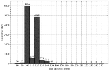
Figure A.3 Distribution of slab thickness

Reference

Alcaide-Marzal, J., Diego-Mas, J.A., 2025. Computers as co-creative assistants. A comparative study on the use of text-to-image AI models for computer aided conceptual design. Computers in Industry 164, 104168. https://doi.org/10.1016/j.compind.2024.104168

Chang, K.-H., Cheng, C.-Y., 2020. Learning to Simulate and Design for Structural Engineering, in: Proceedings of the 37th International Conference on Machine Learning. Presented at the International Conference on Machine Learning, PMLR, pp. 1426–1436.

Dhariwal, P., Nichol, A., 2021. Diffusion Models Beat GANs on Image Synthesis. https://doi.org/10.48550/arXiv.2105.05233

Fei, Y.F., Liao, W.J., Huang, Y.L., Lu, X.Z., 2022a. Knowledge-enhanced generative adversarial networks for schematic design of framed tube structures. Automation in Construction 144, 104619. https://doi.org/10.1016/j.autcon.2022.104619

Fei, Y.F., Liao, W.J., Zhang, S., Yin, P.F., Han, B., Zhao, P.J., Chen, X.Y., Lu, X.Z., 2022b. Integrated Schematic Design Method for Shear Wall Structures: A Practical Application of Generative Adversarial Networks. Buildings 12, 1295. https://doi.org/10.3390/buildings12091295

Fu, B.C., Gao, Y.Q., Wang, W., 2023. Dual generative adversarial networks for automated component layout design of steel frame-brace structures. Automation in Construction 146, 104661. https://doi.org/10.1016/j.autcon.2022.104661

Gu, Y., Huang, Y.L., Liao, W.J., Lu, X.Z., 2024. Intelligent design of shear wall layout based on diffusion models. Computer-Aided Civil and Infrastructure Engineering. https://doi.org/10.1111/mice.13236

Han, J., Lu, X.Z., Gu, Y., Liao, W.J., Cai, Q., Xue, H.J., 2024. Optimized data representation and understanding method for the intelligent design of shear wall structures. Engineering Structures 315, 118500. https://doi.org/10.1016/j.engstruct.2024.118500

Ho, J., Jain, A., Abbeel, P., 2020. Denoising Diffusion Probabilistic Models. https://doi.org/10.48550/arXiv.2006.11239

Iranmanesh A. & Kaveh A., 1999. Structural optimization by gradient base neural networks, International Journal of Numerical Methods in Engineering 46, 297-311. https://doi.org/10.1002/(SICI)1097-0207(19990920)46:2%3C297::AID-NME679%3E3.0.CO;2-C

Kaveh, A., 2024. Applications of artificial neural networks and machine learning in civil engineering. Springer.

Kaveh, A., 2017. Applications of metaheuristic optimization algorithms in civil engineering. Springer.

Kaveh A, Ardalani Sh, 2016. Cost and CO2 Emission Optimization of Reinforced Concrete Frames Using ECBO Algorithm. Asian Journal of Civil Engineering 17, 831-858. https://doi.org/10.1007/978-3-319-48012-1_17

Kaveh, A., Hamedani, K.B., Hosseini, S.M., Bakhshpoori, T., 2020a. Optimal design of planar steel frame structures utilizing meta-heuristic optimization algorithms. Structures 25, 335–346. https://doi.org/10.1016/j.istruc.2020.03.032

Kaveh A., Izadifard R.A., Mottaghi L., 2020b. Optimal Design of Planar RC Frames Considering CO2 Emissions Using ECBO, EVPS and PSO Metaheuristic Algorithms, Journal of Building Engineering 28, 101014. https://doi.org/10.1016/j.jobe.2019.101014

Kaveh A., Kalateh-Ahani M. & Fahimi-Farzam M, 2013. Constructability optimal design of reinforced concrete retaining walls using a multi-objective genetic algorithm, Structural Engineering and Mechanics 47, 227-245. https://doi.org/10.12989/sem.2013.47.2.227

Kaveh, A., Khavaninzadeh, N., 2023. Efficient training of two ANNs using four meta-heuristic algorithms for predicting the FRP strength, Structures 52 256-272. https://doi.org/10.1016/j.istruc.2023.03.178

Kaveh A, and Zakian P., 2014. Seismic Design Optimisation of RC Moment Frames and Dual Shear Wall-Frame Structures via CSS Algorithm, Asian Journal of Civil Engineering, 15,435-465.

Li, G., Lu, H.Y., Liu, X., 2010. A hybrid simulated annealing and optimality criteria method for optimum design of RC buildings. Structural Engineering and Mechanics 35, 19–35. https://doi.org/10.12989/sem.2010.35.1.019

Liang, D., Xue, F., 2023. Integrating automated machine learning and interpretability analysis in architecture, engineering and construction industry: A case of identifying failure modes of reinforced concrete shear walls. Computers in Industry 147, 103883. https://doi.org/10.1016/j.compind.2023.103883

Liao, W.J., Huang, Y.L., Zheng, Z., Lu, X.Z., 2022. Intelligent generative structural design method for shear wall building based on “fused-text-image-to-image” generative adversarial networks. Expert Systems with Applications 210, 118530. https://doi.org/10.1016/j.eswa.2022.118530

Liao, W.J., Lu, X.Z., Fei, Y.F., Gu, Y., Huang, Y.L., 2024. Generative AI design for building structures. Automation in Construction 157, 105187. https://doi.org/10.1016/j.autcon.2023.105187

Liao, W.J., Lu, X.Z., Huang, Y.L., Zheng, Z., Lin, Y.Q., 2021. Automated structural design of shear wall residential buildings using generative adversarial networks. Automation in Construction 132, 103931. https://doi.org/10.1016/j.autcon.2021.103931

Liu, H.H., Tian, Q., Yuan, Y., Liu, X.B., Mei, X.H., Kong, Q.Q., Wang, Y.P., Wang, W.W., Wang, Y.X., Plumbley, M.D., 2023. AudioLDM 2: Learning Holistic Audio Generation with Self-supervised Pretraining. https://doi.org/10.48550/arXiv.2308.05734

Lu, X.Z., Liao, W.J., Zhang, Y., Huang, Y.L., 2022. Intelligent structural design of shear wall residence using physics-enhanced generative adversarial networks. Earthquake Engineering & Structural Dynamics 51, 1657–1676. https://doi.org/10.1002/eqe.3632

Mariniello, G., Pastore, T., Bilotta, A., Asprone, D., Cosenza, E., 2022. Seismic pre-dimensioning of irregular concrete frame structures: Mathematical formulation and implementation of a learn-heuristic algorithm. Journal of Building Engineering 46, 103733. https://doi.org/10.1016/j.jobe.2021.103733

MOHURD, 2012. Load Code for the Design of Building Structures (GB 50009-2012).

Mottaghi, L., Izadifard, R. A., & Kaveh, A., 2021. Factors in the relationship between optimal CO2 emission and optimal cost of the RC frames. Periodica Polytechnica Civil Engineering 65, 1-14. https://doi.org/10.3311/PPci.16790

Ning, M., Sangineto, E., Porrello, A., Calderara, S., Cucchiara, R., 2023. Input Perturbation Reduces Exposure Bias in Diffusion Models. https://doi.org/10.48550/arXiv.2301.11706

Peng, B., Flager, F., Barg, S., Fischer, M., 2021. Cost-based optimization of steel frame member sizing and connection type using dimension increasing search. Optimization and Engineering 23, 1525–1558. https://doi.org/10.1007/s11081-021-09665-5

Qin, S.Z., Guan, H., Liao, W.J., Gu, Y., Zheng, Z., Xue, H.J., Lu, X.Z., 2024. Intelligent design and optimization system for shear wall structures based on large language models and generative artificial intelligence. Journal of Building Engineering, 95, 109996. https://doi.org/10.1016/j.jobe.2024.109996

Qin, S.Z., Liao, W.J., Huang, Y.L., Zhang, S.L., Gu, Y., Han, J., Lu, X.Z., 2025. Intelligent design for component size generation in reinforced concrete frame structures using heterogeneous graph neural networks. Automation in Construction 171, 105967. https://doi.org/10.1016/j.autcon.2025.105967

Rombach, R., Blattmann, A., Lorenz, D., Esser, P., Ommer, B., 2022. High-Resolution Image Synthesis with Latent Diffusion Models. https://doi.org/10.48550/arXiv.2112.10752

Saharia, C., Chan, W., Chang, H., Lee, C.A., Ho, J., Salimans, T., Fleet, D.J., Norouzi, M., 2022. Palette: Image-to-Image Diffusion Models. https://doi.org/10.48550/arXiv.2111.05826

Shorten, C., Khoshgoftaar, T.M., 2019. A survey on Image Data Augmentation for Deep Learning. Journal of Big Data 6, 60. https://doi.org/10.1186/s40537-019-0197-0

Trapani, F.D., Sberna, A.P., Marano, G.C., 2022. A genetic algorithm-based framework for seismic retrofitting cost and expected annual loss optimization of non-conforming reinforced concrete frame structures. Computers & Structures 271, 106855. https://doi.org/10.1016/j.compstruc.2022.106855

Wang, L.F., Liu, J.P., Cheng, G.Z., Liu, E., Chen, W., 2023. Constructing a personalized AI assistant for shear wall layout using Stable Diffusion. https://doi.org/10.48550/arXiv.2305.10830

Wei, C.Y., Han, H., Xia, Y., Ji, Z., 2025. TDAD: Self-supervised industrial anomaly detection with a two-stage diffusion model. Computers in Industry 164, 104192. https://doi.org/10.1016/j.compind.2024.104192

Xu, L., Gong, Y.L., 2001. Preliminary Design of Long-Span King-Post Truss Systems with a Genetic Algorithm. Computer-Aided Civil and Infrastructure Engineering 16, 94–105. https://doi.org/10.1111/0885-9507.00216

Xu, L.H., Yan, X.T., Li, Z.X., 2018. Development of BP-based seismic behavior optimization of RC and steel frame structures. Engineering Structures 164, 214–229. https://doi.org/10.1016/j.engstruct.2018.03.012

Zhang, C., Tao, M.X., Wang, C., Yang, C., Fan, J.S., 2024. Differentiable automatic structural optimization using graph deep learning. Advanced Engineering Informatics 60, 102363. https://doi.org/10.1016/j.aei.2024.102363

Zhao, P.J., Liao, W.J., Huang, Y.L., Lu, X.Z., 2023a. Intelligent design of shear wall layout based on attention-enhanced generative adversarial network. Engineering Structures 274, 115170. https://doi.org/10.1016/j.engstruct.2022.115170

Zhao, P.J., Liao, W.J., Huang, Y.L., Lu, X.Z., 2023b. Intelligent design of shear wall layout based on graph neural networks. Advanced Engineering Informatics 55, 101886. https://doi.org/10.1016/j.aei.2023.101886

Zhou, Y., Leng, H., Meng, S.Q., Wu, H., Zhang, Z., 2024. StructDiffusion: End-to-end intelligent shear wall structure layout generation and analysis using diffusion model. Engineering Structures 309, 118068. https://doi.org/10.1016/j.engstruct.2024.118068