An Intelligent Sizing Design Method for Frame-Shear Wall Components in Industrial Parks via Heterogeneous Graph Neural Networks

Jiaoyang Wang ¹, Wenjie Liao ², Shulu Zhang ^1,3,*, Xinzheng Lu ¹, Hao Liang ³, Chi Zhang ³, Zhishan Zhou ²

1 Department of Civil Engineering, Tsinghua University, 100084, Beijing, China

2 School of Civil Engineering, Southwest Jiaotong University, 610031, Sichuan, China

3 China Southwest Architectural Design and Research Institute Co., Ltd., 610041, Chengdu, China

Advanced Engineering Informatics, 2026, 76: 105100. DOI: 10.1016/j.aei.2026.105100.

 

Abstract: Industrial parks have emerged as a rapidly expanding construction sector, where frame-shear wall systems constitute the primary structural form. The mechanical performance of these structures depends critically on the section sizing of their components. However, conventional sizing design approaches rely predominantly on engineers' empirical judgment and iterative finite element analysis, resulting in inefficient workflows that require extensive manual intervention and computational resources. To overcome these limitations, this study proposes an enhanced Heterogeneous Graph Neural Network (HGNN) integrated with Squeeze-and-Excitation (SE) and PairNorm (PN) modules, denoted as SE+PN+HGNN. This improved model is used to assist in the preliminary sizing design of frame-shear wall structures. Specifically, a heterogeneous graph representation method is developed to incorporate load-specific information for key structural members (columns, beams, and shear walls). Furthermore, a dataset comprising 101 heterogeneous graphs derived from real-world engineering projects is established to support model training. Ablation studies demonstrate that the SE+PN+HGNN method reduces the Root Mean Square Error (RMSE) for component sizing prediction by approximately 21% on average compared with the unimproved HGNN, with the reduction for column dimensions approaching 30%. Following a systematic hyperparameter analysis, the optimal model architecture was applied to case studies of three independent building projects. The results indicate that the proposed method achieves over 70% consistency with engineer-designed solutions within a ±15% tolerance. Furthermore, more than 95% of the AI-generated component sizes meet the Chinese code requirements, suggesting that only a limited proportion of components required subsequent engineer-led refinement. Notably, the proposed method is five times more efficient than traditional design paradigms, demonstrating significant potential for practical engineering applications. Nevertheless, its practical engineering application still requires subsequent structural analysis, code-compliance verification, and engineer-led local refinement.

Keywords: Generative AI Design; Heterogeneous graph; Graph neural network; Frame-shear wall structure; Component sizing design

Highlight

1. Characterized frame-shear wall structures with a load-integrated heterogeneous graph representation method.

2. Constructed a heterogeneous graph dataset based on 101 curated real-world structural design samples.

3. Proposed an intelligent design approach for component sizing prediction using SE+PN enhanced HGNN.

1. Introduction

Recently, the proliferation of industrial parks has generated a substantial construction demand. The frame-shear wall structure is the predominant system utilized. The structural design of these facilities is distinguished by two primary characteristics:

(a) Hybrid formalism: Due to the coupling of frames and walls, its design complexity exceeds that of pure frame or shear wall systems ^[1]. Both frame elements and shear wall components should be considered simultaneously in data representation.

(b) Load complexity: Load characteristics are dictated by the building's diverse operational functions. Consequently, the design load profiles are significantly more complex and varied than those typical of standard residential or commercial office buildings.

The geometric dimensions of structural components directly impact the mechanical performance of the entire structure. As a result, the optimal cross-sectional sizing is indispensable to effective structural design workflows ^[2]. Current engineering practice follows an iterative design paradigm: engineers establish preliminary member sizes based on empirical heuristics and handbook formulas, followed by multiple rounds of finite element analysis (FEA) to verify code compliance and refine dimensions. This process typically requires 5-10 design iterations, each involving comprehensive structural analysis under multiple load combinations. This process results in a labor-intensive, time-consuming workflow that significantly limits design efficiency for large-scale or complex projects ^[3]. Consequently, an intelligent cross-sectional design methodology is required to streamline workflows and enhance the engineers' design efficiency.

To address these challenges, existing research has leveraged metaheuristic algorithms for automated structural design. A wide range of optimization techniques—including Simulated Annealing (SA) ^{[4, 5]}, Genetic Algorithms (GA) ^[6], Particle Swarm Optimization (PSO) ^[7], Plasma Generation Optimization (PGO) ^[8], Heap-based Optimizer (HBO) ^[9], and Teaching-Learning-Based Optimization (TLBO) ^[10]—have been applied within civil engineering. However, these metaheuristic-driven methods usually require a robust initial design, which significantly limits their practical applicability.

With the advancement of Machine Learning (ML), traditional algorithms such as Decision Tree (DT) and Support Vector Machine (SVM) have also been adopted in this domain ^{[11, 12]}. More recently, the emergence of Deep Learning (DL) has further enabled the realization of intelligent design paradigms^[13]. For instance, Generative Adversarial Networks (GANs) have been successfully applied to both architectural ^[14] and structural design tasks ^[15]. Meanwhile, the diffusion model has also been investigated for similar applications ^[16]. Furthermore, in physics-informed integration, a framework combining the finite element method with deep reinforcement learning, called FrameRL, was developed to enable intelligent design of steel frame structures ^[17]. Despite these diverse approaches, recent research indicates that intelligent structural design, particularly when facilitated by advances in Graph Neural Networks (GNNs), achieves superior performance through graph-based representations ^[18].

As data structures composed of nodes and edges, graphs align topologically with physical systems, allowing for the intuitive characterization of civil engineering structures. Consequently, graph representations have been widely adopted in computational mechanics and engineering ^[19]. By leveraging both graph data structures and neural architectures, Graph Neural Networks (GNNs) have experienced a surge in popularity within the machine learning community ^[20]. Demonstrating the capability of GNNs in structural scheme design, Zhao et al. proposed a framework that converts shear wall structures into graph data to effectively extract topological features and guide layout generation ^[21]. Fei et al. proposed a GNN-integrated evolutionary framework employing a distance-based updating strategy to efficiently correct surrogate prediction errors without retraining ^[22]. Nourian et al. proposed a framework that combines a GNN with Particle Swarm Optimization (PSO) ^[23]. Additionally, Li et al. combined GNN with an enhanced genetic algorithm (EGA) to automate reinforcement design and collision detection ^[24]. Enhancing the applicability of graph-based methods, Zhao et al. introduced an innovative GNN framework that accounts for specific structural conditions—including peak ground acceleration and building height—thereby improving the reliability of the generated designs ^[25]. Similarly, Ruan et al. integrated physics-informed constraints into GNN model to infer the internal states of reinforced concrete (RC) frames, achieving performance superior to traditional GNN ^[26].

In contrast to homogeneous GNN, heterogeneous graph neural networks (HGNNs) can incorporate diverse node types and attributes, offering enhanced scalability and practicality ^[27]. Qin et al. leveraged HGNN to automatically generate cross-sectional sizes for structural components (e.g., beams, columns, and slabs) in RC frames, significantly streamlining the design process ^[28]. In civil engineering, Li et al. proposed "StructureGraph", an HGNN-based model for automotive structural design, achieving robust results and demonstrating the strong generalization capabilities of HGNN across various engineering domains ^[29]. Concurrently, Tian et al. explored HGNN applications within the civil engineering informatics domain, contributing a novel approach to leverage heterogeneous graph representations for engineering design tasks ^[30].

However, existing research still exhibits certain limitations, primarily manifested in the following aspects:

(a) AI training heavily relies on a high-quality dataset. For the sizing design of industrial park buildings, load data plays a critical role. Nevertheless, as noted by Urbieta et al., practical labeled datasets are predominantly generated from visual construction drawings, which typically fail to capture essential load-bearing details ^[31]. In addition, some scholars have made efforts to address this issue. Hou et al. proposed a graph structure descriptor based on boundary representation (B-rep graph) and an efficient graph convolutional network (FuS-GCN) for the classification and retrieval of 3D-CAD models, providing a feasible solution for the efficient reuse of CAD models in industrial manufacturing ^[32]. Teng et al. introduced a self-supervised heterogeneous graph attention model (HGAM) that employs adaptable step-size metapaths and dual contrastive learning, eliminating the need for predefined metapaths and alleviating the scarcity of labeled data in complex graphs ^[33].

(b) Currently, most generative design studies focus on frame structures and shear wall structures, while frame-shear wall structures have received limited attention. From the structural layout perspective, the diversity of building functions results in substantial variations in the configuration of frame-shear wall structures. From a mechanical analysis perspective, a complex challenge is balancing the stiffness and bearing capacity of frames and shear walls in such dual systems.

(c) Existing unimproved HGNN models exhibit suboptimal regression prediction performance on multi-class heterogeneous graphs ^[34]. Consequently, the application of HGNNs to predict the cross-sectional dimensions of diverse frame components remains limited.

To address the aforementioned limitations, this study proposes an intelligent cross-sectional sizing model for frame-shear wall structural components. This model is based on an HGNN architecture enhanced by the integration of squeeze-and-excitation (SE) and PairNorm (PN) modules. Specifically, the SE module is utilized to enhance the model's flexibility in learning heterogeneous graph features through a channel-wise attention mechanism ^[35]. Concurrently, the PN module addresses oversmoothing in deep GNN by ensuring that distant nodes retain dissimilar features ^[36]. By incorporating heterogeneous graphs of frame-shear wall structures with multi-class nodes and edges that contain detailed load information, the proposed framework enables the end-to-end generation of component cross-sectional sizes.

2. HGNN-based design methodology

The proposed framework for designing cross-sectional sizes of frame-shear wall structural components is illustrated in Figure 1. The framework comprises three specific steps: dataset generation, model training, validation and hyperparameter selection, and case studies.

(a) Dataset generation: This study proposes a novel heterogeneous graph representation for industrial park buildings with frame-shear wall structures. In this proposed graph, detailed load information is explicitly encoded as a known node attribute. The methodology entails the manual annotation of computer-aided design (CAD) drawings and their subsequent preprocessing into a heterogeneous graph format compatible with computational analysis. Derived from real-world engineering projects, a final dataset comprising 101 heterogeneous graph instances was constructed. This process will be detailed in Section 3.

(b) SE+PN improved HGNN model training, validation, and hyperparameter selection: Current HGNN models demonstrate limitations in handling the multi-class regression task, often resulting in limited accuracy. This study proposes an improved HGNN incorporating SE (Squeeze-and-Excitation) and PN (PairNorm) mechanisms. The proposed network was rigorously trained and validated using the constructed dataset. A comprehensive series of comparative and ablation experiments was subsequently conducted to verify the effectiveness of the model enhancements and to determine the optimal hyperparameters. The results of these experiments and the analyses will be discussed in Sections 4 and 5.

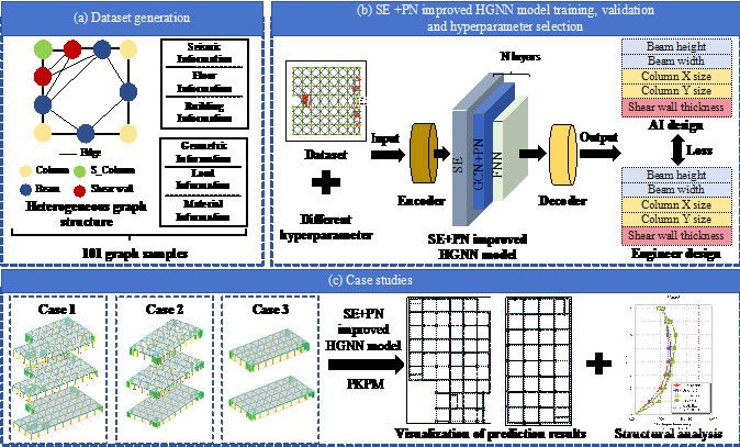
Figure 1. Implementation workflow of frame-shear wall structure dimension design based on HGNN

(c) Case studies: Predictive performance for component sizing was assessed using three structurally distinct buildings, which constituted an independent test set completely separate from the training and validation data. The reliability of the AI-generated data was evaluated through comparative visualization. Additionally, structural analysis software PKPM was employed to calculate seismic mechanical indicators for the three buildings. The analysis indicates that the AI-generated designs generally satisfy the global structural control indices of the Chinese codes, while local component-level violations are further discussed in Section 6.

3. Heterogeneous Graph Representation and Dataset

3.1 Heterogeneous Graph Representation

Graph representation is crucial for HGNNs, significantly influencing their predictive performance ^[37]. In frame-shear wall structures, beams and columns are typically modeled as one-dimensional members (where the width and height are significantly smaller than the length), whereas shear walls are treated as two-dimensional elements (with the length and height of comparable scale, both substantially greater than the thickness). This disparity results in a more complex topological relationship, making the construction of an accurate heterogeneous graph representation for such systems critically important.

During structural design, the slab thickness is primarily governed by the effective span and the applied load conditions. Given the narrow range of feasible options, the appropriate size can be readily determined using established algorithms. Additionally, secondary beams and semi-frame beams (i.e., beams supported by a column at one end and a primary frame beam at the other) serve mainly to shorten the effective slab span and transfer partition wall loads. Their cross-sections are likewise dictated by loading and span. Consequently, to streamline the intelligent design process, this study concentrates on the primary load-bearing elements, specifically shear walls, frame columns, and frame beams. For the cross-sectional design of frame-shear wall structures, secondary components, including slabs, secondary beams, and semi-frame beams, are excluded from the scope.

A common approach to structural graph representation involves modeling structural components as nodes and their interconnections as edges ^[38]. The heterogeneous graph representation employed in this study is depicted in Figure 2. It consists of four types of nodes, frame columns, frame beams, shear walls, and shear wall end columns (S_Columns). These nodes are interconnected through six distinct edge types. This formalism abstracts the frame-shear wall structure into a computationally interpretable heterogeneous graph, thereby enabling its processing with HGNN for subsequent learning and prediction tasks.

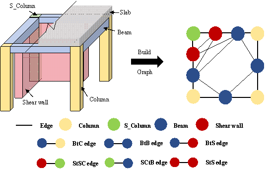
Figure 2. Heterogeneous graph representation

As illustrated in Figure 2, each individual shear wall segment is modeled as a distinct node in the graph representation. This modeling approach is motivated by the fact that, in engineering practice, a single shear wall is frequently comprised of interconnected segments, which often form complex non-planar configurations such as L-shaped or T-shaped sections. Furthermore, a shear wall end column (S_Column) often functions integrally with the shear wall as a combined load-resisting system in the actual design. However, its design principles differ from those of frame columns. Consequently, the proposed graph representation explicitly distinguishes between these two member types. It is important to note that the shear wall end column (S_Column) serves only as an intermediate data category to differentiate between column types and is excluded from the final statistical metrics of structural components.

3.2 Heterogeneous Graph Information

The heterogeneous graph proposed in this study integrates information from both CAD drawings and overall design parameters. As illustrated in Figure 3, geometric, load, and material properties are retrieved from the CAD drawings, while seismic information, floor information, as well as other global information are sourced from the engineer's foundational input. Referring to the studies by Zhao et al. (2023) ^[25] and Yu et al. (2025) ^[39], all specific attributes in the graph are summarized in Table 1 and used as direct inputs to the model.

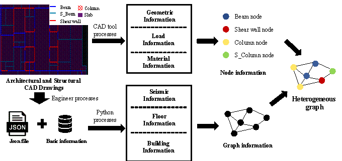
Figure 3. Information sources of the heterogeneous graph

Table 1. Details of the heterogeneous graph information

Information category	Information composition
Geometric Information	Relative X coordinate, relative Y coordinate, X-axis length of drawing, Y-axis length of drawing, Component length, orientation
Load Information	Live load, dead load, max live load, max dead load
Material Information	Material strength
Seismic Information	Peak ground acceleration (PGA), site condition, seismic design group, seismic fortification intensity, design characteristic period
Floor Information	Floor height, relative floor position, Total number of floors, current number of labeled floors
Building Information	Structural type, building use type

Each type of node in the heterogeneous graph possesses the feature categories listed in Table 1. Edge attributes are defined by the pair of linked nodes, with the construction method specified in Equation (1).

(1)

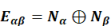
where  denotes the edge connecting nodes  and ,  denotes the feature vector of node , and  denotes the feature vector of node .

A critical enhancement introduced in this study involves the explicit incorporation of detailed load information for each structural component. Loads are assigned based on member length, an approach that simplifies computation without significantly compromising accuracy ^[40]. The specific load values are determined by tracing the complete load path through the structural hierarchy: from slabs, to secondary beams or shear walls, and finally to main frame columns or shear wall end columns (S_Columns). However, the substantial variation in load magnitudes typical of industrial park buildings can impede model convergence. To mitigate this issue, the load data are normalized using Equation (2), a technique proven to enhance data quality and facilitate neural network training.

(2)

_{where  and  are the dead load and live load of the i-th component,  and  denote the normalized dead load and live load, and  is the number of components in the current graph.}

3.3 Dataset Construction

The methodology involves the meticulous preprocessing of engineering drawings to generate a heterogeneous graph representation compatible with the HGNN architecture. Since secondary and semi-frame beams (excluded from the final graph) disrupt structural connectivity in the original data, preprocessing is required to merge primary members and restore connections, as outlined in Figure 4.

The quality of the dataset is crucial to model training. A high-quality dataset derived from real-world engineering can significantly improve model generalization. Therefore, this study curates a dataset of 101 representative industrial park frame-shear wall structures by applying denoising techniques and manual selection. This dataset was partitioned into training, validation, and test sets using a conventional split ratio of 6:2:2. The statistical distribution of component sizes within the heterogeneous graph dataset is presented in Figure 5. It shows that frame beam sections predominantly measure 800 mm in height by 300 mm in width, frame column dimensions mostly measure 700 mm × 700 mm, and shear wall thickness is mostly 300 mm.

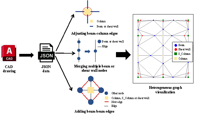
Figure 4. Preprocessing workflow for heterogeneous graph construction

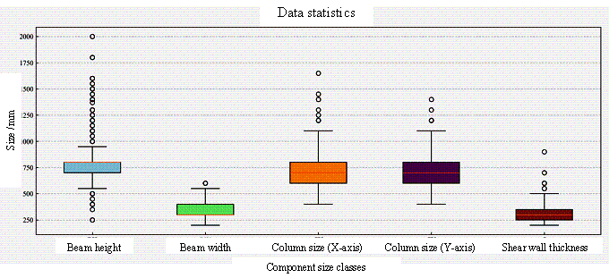
Figure 5. Overview of cross-sectional size statistics for structural components in the dataset

4. SE+PN Enhanced HGNN Architecture

Shown in Figure 6, a novel HGNN model was constructed based on Qin et al. ^[28] to process the heterogeneous graph representations of frame-shear wall structures. Notably, this model introduces SE modules between the encoder and the graph convolutional network (GCN)^[41] to enhance the model. Meanwhile, a PN module is added to the GCN framework. This approach differs from the work of Qin et al. ^[28] in the following two aspects:

(a) To address the variety of node categories in the constructed heterogeneous graph, the SE module is incorporated into the neural network ^[35]. This enhancement enables the model to adaptively weigh different data types, thereby improving its predictive performance.

(b) To alleviate the issue of oversmoothing in graph representations, this study integrates the PN module ^[36] into the GCN to prevent excessive smoothing of information.

The architecture of the proposed heterogeneous graph neural network adopts an n-layer GCN as its backbone, supplemented by an encoder and a decoder for preliminary graph encoding and final data decoding. This design enables the network to process the input heterogeneous graph sequentially: the graph is first encoded, subsequently passed through the enhanced GCN for feature aggregation and prediction, and finally decoded to output the predicted cross-sectional sizing of the frame-shear wall structural components.

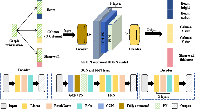
Figure 6. Architecture of the SE+PN enhanced HGNN model

Specifically, the SE is applied between the encoder and the GCN backbone, where separate SE modules are used to recalibrate features for each node category. Following the design of common architectures, the PN module is incorporated into the GCN to process the resulting features and preserve gradient information across the graph.

All model training and prediction experiments were performed on an RTX 3050Ti GPU, operating within a standardized computational environment configured with PyTorch 2.2.0 and CUDA 12.6. As detailed in Algorithm 1, training the proposed HGNN model primarily involves three stages: dataset splitting, training, and validation. During data processing, it is noteworthy that the graph features are directly concatenated with the node information to form a feature vector that encompasses all attributes listed in Table 1, which is then fed as input to the model.

Algorithm 1 Training

input graph_info, node_info, config     # get subgraph from original information     info = graph_info ⊕ node_info     subgraph = create_subgraph(info)     train_dataset, val_dataset, test_dataset = divide_data(subgraph)     # model train     HGNN = get_model(config)     for epoch in config.epochs do:         fet = get_feature(train_dataset, config)         HGNN.train(fet, aggregate="sum")     end for     # model val     HGNN.eval ( )     fet = get_feature(val_dataset, config)     RMSE, MRE = HGNN.val(fet, aggregate="sum") output RMSE, MRE

The core of graph neural networks lies in the message-passing mechanism, which iteratively aggregates information from neighboring nodes to update the representation of the target node. In heterogeneous graphs, where both nodes and edges can be of multiple types, the message-passing process must distinguish among edge types to learn structure-dependent semantic information. However, in practical structural systems, the force transmission patterns among components are similar. Consequently, the six edge types in this study use similar propagation functions, resulting in relatively weak heterogeneity at the relation level. Therefore, the heterogeneity of this work is primarily reflected in node heterogeneity.

For a given node , the message-passing function at the -th layer is expressed as shown in Equation (3). This formula embodies a relation-aware aggregation strategy in which each edge type independently learns feature transformations, and multi-source information is ultimately fused via summation.

(3)

where  represents the neighbors of node  under relation ,  and  are the relation-specific learnable weight matrix and bias term, respectively, and  and  are node degree normalization coefficients, and  means activation function (e.g. ReLU function).

The mean squared error (MSE) loss function is adopted, and its mathematical formulation is presented in Equation (4).

(4)

where  denotes the set of node types present in the graph;  is the number of nodes of type ,  represents the prediction dimension for type  (with a value of 2 for beams and columns, and 1 for shear walls);  is the engineer‑designed value of the -th dimension for the -th node of type ; and  is the corresponding predicted value.

5. Discussion

5.1 Evaluation Metrics

The accuracy of the neural network predictions is quantified by the consistency between model outputs and actual cross-sectional data, using the Root Mean Square Error (RMSE) and Mean Relative Error (MRE) as evaluation metrics. RMSE is a prevalent error metric in deep learning, favored for its sensitivity to large deviations and its scale-consistency with the predicted values, which facilitates direct interpretation. In contrast, the MRE is better suited to reflecting the model's overall performance, as it focuses on relative error.

On the validation set, RMSE is used to evaluate the deviation between the predicted and actual component dimensions. Given that relative errors are more meaningful for engineering comparison, MRE is also adopted for validation-set-based model selection. The test set is reserved for final evaluation after the model configuration is fixed. The formulas for RMSE and MRE are shown in Equations (5) and (6), respectively.

	(5)
	(6)

where  is the total number of samples in the dataset,  is the engineer‑designed value of the i-th sample, and  is the predicted value of the i-th sample.

5.2 Ablation Study

An ablation study was conducted to validate the proposed model. To ensure objectivity and accuracy, the experimental setup, determined through pre-training, was as follows: 300 epochs, a learning rate of 0.01, two GCN layers, 30 hidden layer features, and a batch size of 16. Detailed metrics from this experiment are provided in Tables 2 and 3.

The results indicate that, compared with the original HGNN model, the introduction of the SE and PN modules improves the RMSE performance for several structural dimension prediction tasks. In particular, SE+PN+HGNN achieves the lowest RMSE for beam height, column X dimension, and column Y dimension, suggesting that the joint use of the two modules enhances the model’s ability to represent key structural features. Therefore, considering the validation results and engineering relevance, SE+PN+HGNN is selected as the improved model.

Table 2. RMSE results on the validation set from the ablation study

Model description	Beam height RMSE (mm)	Beam width RMSE (mm)	Column X dimension RMSE (mm)	Column Y dimension RMSE (mm)	Shear wall thickness RMSE (mm)
HGNN	164.56	65.02	145.05	155.19	62.60
PN+HGNN	134.43	65.27	108.49	123.16	64.99
SE+HGNN	135.04	78.63	116.64	124.20	61.29
SE+PN+HGNN	129.27	65.23	103.77	108.93	62.65

In terms of module effectiveness, the PN module improves feature normalization and propagation during graph convolution, which helps alleviate feature over-smoothing caused by multi-layer information aggregation and better preserves the differences among structural component nodes. Compared with the original HGNN, PN+HGNN substantially reduces the RMSE for beam height and column dimensions, indicating that PN effectively enhances the model’s ability to identify key component dimension features.

The SE module further strengthens the model’s attention to important channel features through feature recalibration, enabling the model to better utilize effective information related to structural dimension prediction. The combination of SE and PN further improves the representation capability of the model, demonstrating the effectiveness of the two modules in enhancing the original HGNN.

Table 3. MRE results from the ablation study on the validation set

Model description	HGNN	PN+HGNN	SE+HGNN	SE+PN+HGNN
MRE	12.73%	12.36%	10.96%	11.92%

As shown in Table 3, SE+HGNN achieves the lowest MRE on the validation set, indicating that the SE module effectively improves the overall prediction accuracy of the model. Although SE+PN+HGNN does not achieve the lowest MRE on the validation set, its prediction error remains lower than that of the original HGNN, demonstrating that the combined use of the SE and PN modules improves the model’s capability for structural dimension prediction.

5.3 Hyperparameter Selection

To ensure reproducibility, the hyperparameter search space and final selections are listed in Table 4. These ranges were determined based on preliminary experiments and domain knowledge to examine the influence of key hyperparameters on model performance. SE+PN+HGNN-H30-L0.01-G2 was used as a common baseline for the GCN-layer, graph-representation, and robustness analyses to ensure consistent comparison settings. However, this baseline was not directly selected as the final model. The final configuration was determined by further balancing validation performance and model complexity, as discussed in Section 5.3.1 and applied in Section 6.

Table 4. Hyperparameter search space and final selection

5.3.1 Influence of Different Configurations of Hidden Features and Learning Rates

Selecting appropriate values for the number of hidden layers and the learning rate is essential for model performance. To identify the optimal configuration, experiments with a fixed batch size of 16 across 300 epochs are conducted. The corresponding RMSE and MRE metrics are summarized in Tables 5 and 6.

Table 5. RMSE results on the validation set for different numbers of hidden features and learning rates

Experimental setup	Beam height RMSE (mm)	Beam width RMSE (mm)	Column X dimension RMSE (mm)	Column Y dimension RMSE (mm)	Shear wall thickness RMSE (mm)
SE+PN+HGNN-H10-L0.01	536.56	157.59	285.47	272.85	68.33
SE+PN+HGNN-H20-L0.01	130.24	64.40	104.35	114.91	65.30
SE+PN+HGNN-H30-L0.01	129.27	65.23	103.77	108.93	62.65
SE+PN+HGNN-H40-L0.01	131.69	63.16	117.29	125.79	70.66
SE+PN+HGNN-H50-L0.01	126.88	63.38	124.71	154.83	67.03
SE+PN+HGNN-H30-L0.0075	185.95	63.77	98.54	107.03	69.03
SE+PN+HGNN-H30-L0.0125	129.26	63.69	128.44	145.47	64.18

* In the table, H denotes the number of hidden features, and L denotes the learning rate.

Table 5 shows that the number of hidden features has a direct impact on the model performance. With only 10 hidden features, the model produces much larger RMSE values, indicating that too few hidden features limit its representation capacity and weaken its ability to learn structural relationships. As the number of hidden features increases, the prediction accuracy improves substantially. However, further increasing the hidden feature dimension does not consistently improve the results, suggesting that excessive hidden features may introduce redundant parameters and reduce optimization efficiency. For the learning rate, 0.01 provides more balanced performance than 0.0075 and 0.0125 across different structural dimension prediction tasks.

As shown in Table 6, SE+PN+HGNN-H30-L0.0075 achieves the lowest MRE on the validation set, followed closely by SE+PN+HGNN-H30-L0.01. Considering the balance between validation accuracy and model complexity, SE+PN+HGNN-H20-L0.01 was selected as the final configuration. Although it does not achieve the lowest MRE, its performance is close to the best-performing configuration while using fewer hidden features, making it more suitable for the subsequent case studies. Overall, the results indicate that a moderate hidden-feature dimension is more suitable for balancing model capacity and prediction accuracy.

Table 6. MRE results on the validation set for different numbers of hidden features and learning rates

Experimental setup	SE+PN+HGNN-H10-L0.01	SE+PN+HGNN-H20-L0.01	SE+PN+HGNN-H30-L0.01	SE+PN+HGNN-H40-L0.01	SE+PN+HGNN-H50-L0.01	SE+PN+HGNN-H30-L0.0075	SE+PN+HGNN-H30-L0.0125
MRE	26.45%	12.07%	11.92%	12.74%	13.56%	11.81%	13.70%

5.3.2 Influence of GCN Layers

Selecting an appropriate model depth is critical for effective learning. To this end, the optimal number of GCN layers was investigated by configuring the SE+PN enhanced HGNN with 2, 3, and 4 layers. All experiments used a fixed batch size of 16 and were trained for 300 epochs. The corresponding RMSE results are presented in Table 7.

As shown in Table 7, the two-layer GCN achieves the lowest RMSE for beam height, column Y dimension, and shear wall thickness, showing stable overall performance. The four-layer GCN performs better in predicting beam width and column X dimension, while the three-layer GCN gives relatively poorer results. This indicates that increasing the number of GCN layers does not always improve prediction accuracy and may cause redundant information or feature over-smoothing.

Table 7. RMSE results on the validation set for different numbers of GCN layers

Experimental setup	Beam height RMSE (mm)	Beam width RMSE (mm)	Column X dimension RMSE (mm)	Column Y dimension RMSE (mm)	Shear wall thickness RMSE (mm)
SE+PN+HGNN-H30-L0.01-G2	129.27	65.23	103.77	108.93	62.65
SE+PN+HGNN-H30-L0.01-G3	142.04	66.16	125.50	132.93	66.72
SE+PN+HGNN-H30-L0.01-G4	138.18	59.52	107.78	114.36	66.65

* H denotes the number of hidden features, L denotes the learning rate, and G denotes the number of GCN layers.

As shown in Table 8, SE+PN+HGNN-H30-L0.01-G2 achieves the lowest MRE on the validation set. As the number of GCN layers increases, the MRE also increases. Therefore, the two-layer GCN is selected because it provides a better balance between prediction accuracy and model stability.

Table 8. MRE results on the validation set for different numbers of GCN layers

Experimental setup	SE+PN+HGNN-H30-L0.01-G2	SE+PN+HGNN-H30-L0.01-G3	SE+PN+HGNN-H30-L0.01-G4
MRE	11.92%	12.80%	13.16%

5.4 Comparative Experiments on Heterogeneous Graph Representations

The choice of heterogeneous graph representation significantly determines model training efficacy. To leverage this, we employ an optimal structure to improve the performance of the SE+PN enhanced HGNN. A comparative study of the three graph representations presented in Figure 7 serves to validate our design choices: GraphType-1 (basic frame: columns, beams, shear walls); GraphType-2 (adds shear wall end columns, S_Columns); GraphType-3 (expands shear wall connectivity). All experiments used the improved HGNN (learning rate: 0.01, hidden features: 30, GCN layers: 2, batch size: 16, epochs: 300). The resulting RMSE metrics are in Table 9.

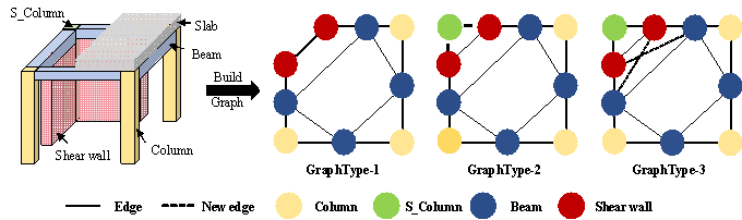
Figure 7. Heterogeneous graph representations of different experimental groups

Table 9. RMSE results on the validation set for different heterogeneous graph representations

Graph types	Beam height RMSE (mm)	Beam width RMSE (mm)	Column X dimension RMSE (mm)	Column Y dimension RMSE (mm)	Shear wall thickness RMSE (mm)
GraphType-1	130.38	63.83	107.42	115.44	69.92
GraphType-2	133.07	65.22	103.78	119.20	62.36
GraphType-3	129.27	65.23	103.77	108.93	62.65

Table 10. MRE results on the validation set for different heterogeneous graph representations

Graph types	GraphType-1	GraphType-2	GraphType-3
MRE	12.27%	12.43%	11.92%

As listed in Table 9, different heterogeneous graph representations lead to different prediction performance across structural components. GraphType-1 achieves relatively good performance for beam width, but its errors for column dimensions and shear wall thickness are higher. GraphType-2 improves the prediction of shear wall thickness and obtains competitive results for column X dimension, but its performance for beam components and column Y dimension is less favorable. In comparison, GraphType-3 achieves the lowest RMSE for beam height and both column dimensions, while maintaining a comparable error for shear wall thickness. This indicates that GraphType-3 provides a more balanced graph representation and better captures the relationships among beams, columns, and shear walls. Therefore, GraphType-3 shows the best overall performance among the evaluated graph representations.

As shown in Table 10, among the three heterogeneous graph representations, GraphType-3 achieves the lowest MRE on the validation set. This also suggests that GraphType-3 can more effectively represent the structural relationships among different component types.

5.5 SOTA Comparison

In this task, four state-of-the-art (SOTA) models were selected for training using the same hyperparameter configuration as in the ablation study: 300 epochs, a learning rate of 0.01, and a batch size of 16. Homogeneous GCN ^[41] and GAT ^[42] models are also employed to demonstrate the superiority of heterogeneous networks in this project. Additionally, HGT ^[44] and HAN ^[43], two widely used heterogeneous models in recent years, were also included for comparison. All SOTA models were evaluated on the fixed independent test set to compare their generalization performance. The results are presented in Tables 11 and 12.

Table 11. RMSE results on the test set from the SOTA comparison

Model description	Beam height RMSE (mm)	Beam width RMSE (mm)	Column X dimension RMSE (mm)	Column Y dimension RMSE (mm)	Shear wall thickness RMSE (mm)	Mean RMSE (mm)
GCN[41] (homogeneous)	193.04	129.72	191.68	202.56	76.44	158.69
GAT [42] (homogeneous)	137.16	105.07	169.63	170.22	65.39	129.49
HAN [43]	131.39	104.43	182.03	184.43	40.85	128.63
HGT [44]	147.74	103.28	149.88	150.31	45.41	119.32
SE+PN+HGNN-H30-G2	122.49	107.41	133.84	135.23	49.43	109.68
SE+PN+HGNN-H20-G2	118.34	101.02	96.53	101.52	54.34	94.35

* H denotes the number of hidden features, L denotes the learning rate, and G denotes the number of GCN layers

Table 12. MRE results on the test set from the SOTA comparison study

Model description	GCN[41](homogeneous)	GAT[42](homogeneous)	HAN[43]	HGT[44]	SE+PN+HGNN-H30-G2	SE+PN+HGNN-H20-G2
MRE	17.91%	15.51%	14.22%	13.35%	13.30%	11.62%

As shown in Tables 11 and 12, the SE+PN+HGNN-H20-G2 model achieves the lowest RMSE and MRE among all compared methods, demonstrating superior overall prediction accuracy across the five geometric components—particularly in beam dimensions. In addition, SE+PN+HGNN-H30-G2, serving as a baseline for comparison, also shows improved performance over the four SOTA models. Heterogeneous architectures consistently outperform homogeneous ones on the evaluation metrics. This underscores that heterogeneous graph neural networks, or the proposed networks, are better equipped to learn and capture the characteristics of real-world structures. Moreover, the proposed model also achieves a lower mean RMSE than other SOTA methods, confirming its architectural superiority.

5.6 Five-Fold Cross-Validation

To evaluate the influence of random seeds and the robustness of the model, five-fold cross-validation experiments are conducted under five different random seeds. For each random seed, 20% of the data was held out as an independent test set. Five-fold cross-validation was then performed only on the remaining 80% development data. Model stability was assessed on validation folds, and the independent test set was used only after the model configuration was fixed.

The mean and standard deviation of the RMSE for the predicted dimensions of each component on the validation sets are reported in Table 13, while the corresponding results on the independent test set are presented in Table 14. Additionally, the overall coefficients of variation (CV) across the five random seeds are summarized in Table 15. These experiments are conducted using the SE+PN+HGNN-H30-G2 model, with the following hyperparameters: a learning rate of 0.01, 300 training epochs, and a batch size of 16. It should be clarified that SE+PN+HGNN-H30-L0.01-G2 is adopted as a common baseline configuration for the subsequent GCN-layer, graph-representation, and robustness analyses. This setting is used only for comparative consistency and is not involved in the final model-selection process.

Table 13. Five-fold cross-validation RMSE results on validation set for different random seeds

* Results are presented as mean ± standard deviation

As shown in Table 13, the RMSE results obtained from five-fold cross-validation under different random seeds remain generally stable for the predicted dimensions of all structural components. No significant abnormal fluctuations are observed for beam height, beam width, column dimensions, or shear wall thickness, indicating that the model is robust to random data partitioning and parameter initialization. Among these components, the prediction of beam width exhibits the highest stability, suggesting that the model can effectively capture its dimensional distribution. In contrast, the errors for beam height and column dimensions show relatively larger variations, which may be attributed to their stronger dependence on structural layout, loading conditions, and engineering constraints. Overall, the SE+PN+HGNN-H30-G2 model maintains consistent predictive performance across different random seeds, demonstrating the stability and reliability of the proposed method on the validation sets.

As shown in Table 14, the mean RMSE values for structural dimension prediction on the independent test set are relatively consistent across the five random seeds, indicating stable predictive performance on unseen data. The CV values in Table 15 remain low for most prediction metrics, with only minor variations observed across different seeds. This suggests that the generalization performance of the model is not sensitive to random initialization or data partitioning. In addition, the limited fluctuation in test-set RMSE indicates that the model does not rely on a specific training split to achieve satisfactory performance. Overall, these results demonstrate that the proposed model has reliable generalization capability and robustness when applied to unseen structural design samples.

Table 14. Five-fold cross-validation RMSE results on held-out test set for different random seeds

* Results are presented as mean ± standard deviation

Table 15. Five-fold cross-validation CV results on held-out test set

6. Case studies

6.1 Cases Description

It should be noted that SE+PN+HGNN-H30-L0.01-G2 was used as a common baseline for the GCN-layer, graph-representation, and robustness analyses to ensure consistent comparison settings. However, this configuration was not selected as the final model. After comparing the validation results and model complexity, SE+PN+HGNN-H20-L0.01-G2 was chosen for the case studies because it achieved comparable performance with fewer hidden features.

To further examine the validity of the proposed model's predictions, three representative structures of high-rise industrial park buildings, excluded from both the training and validation sets, were selected for analysis. The design parameters of each structure are: seismic design intensity is 7 degrees (the corresponding peak ground acceleration under the design basic earthquake level (DBE) is 0.10 g (probability of exceedance of 10% in 50 years)), and site characteristic period (T_g) is 0.40 s, according to the Code for Seismic Design of Buildings (GB/T 50011-2010). A summary of the basic engineering characteristics for Case 1 through Case 3 is presented in Figure 8.

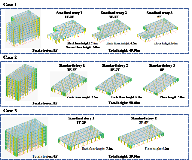
Figure 8. Basic information of the three case-study buildings

6.2 Results of AI-Based Design on Case Studies

Professional structural design adheres to well-established heuristics, among which geometric symmetry serves as a fundamental principle for ensuring balanced load distribution and predictable seismic response. To evaluate whether AI-generated designs conform to these engineering norms, these studies employ a visual analysis approach that encodes cross-sectional dimensions through color and geometric attributes:

(a) Beams: Rectangle width denotes beam width; color encodes beam depth.

(b) Columns: Column sections are identified by distinct color codes. The X and Y-side lengths of the displayed rectangles represent the corresponding cross-sectional dimensions.

(c) Shear walls: Both color and width of the rectangle represent wall thickness.

Furthermore, to avoid visual confusion between beams and walls in the representation, distinctly different color schemes are intentionally adopted for differentiation. The visualization results of the component cross-sectional sizing designed by the SE+PN improved HGNN model are presented in Figures 9 (a), (b), and (c).

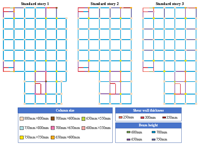
(a) Case 1

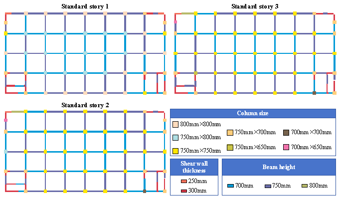
(b) Case 2

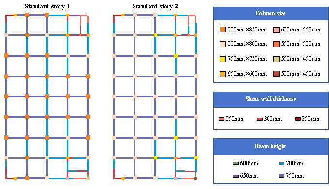
(c) Case 3

Figure 9. Visualization of the AI-generated cross-sectional sizing results

As shown in Figure 9, the component sizes predicted by the proposed model generally satisfy symmetry requirements, meaning that components at symmetrical positions do not exhibit significant dimensional discrepancies. This indicates that the proposed model can effectively learn from the design experience of engineers. Furthermore, the visualization results suggest that the cross-sectional sizing generated by the intelligent design exhibits good consistency across sections.

6.3 Comparative Case Studies: Results and Discussion

On this basis, a comparative analysis was conducted to evaluate the feasibility of the intelligent design outputs by examining their agreement with real-world engineering cases. During the preliminary design stage, since multiple acceptable solutions can exist for cross-sectional sizing, a relative error threshold of 15% was applied. Outcomes with relative error below this threshold are deemed consistent with the actual designs, whereas those above it are considered significantly divergent. Visual comparisons of the three cases are provided in Figures 10 (a), 10 (b), and 10 (c).

As shown in Figure 10, more than 70% of component predictions deviate by less than 15%. Furthermore, the proposed model demonstrates higher accuracy in predicting shear walls, achieving an accuracy rate of approximately 80%. Subsequent analysis reveals that, although the cross-sectional dimensions differ from those of the original design, the AI-generated drawings meet the global code requirements in most design cases after holistic structural verification with design software. Only a limited number of non-compliant components require minor manual adjustment. This comparative analysis reveals that the model maintains reasonable prediction accuracy but also generates viable design alternatives, demonstrating its emergent generative design capacity.

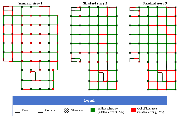
(a) Case 1

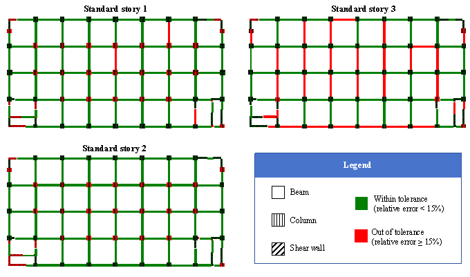
(b) Case 2

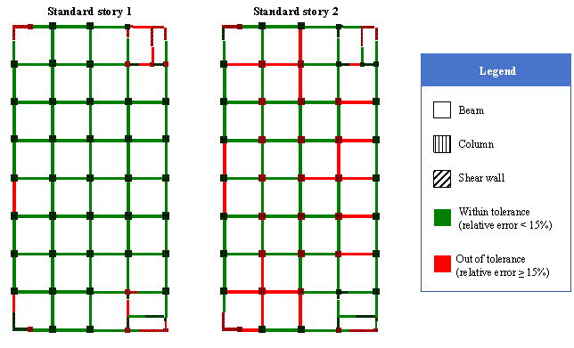
(c) Case 3

Figure 10. Visualization of relative errors in the AI-generated designs

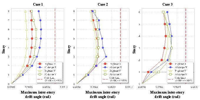
Figure 11. Maximum inter-story drift ratio in the case study

To assess the mechanical performance of the AI-generated designs, performance indicators for the three cases were calculated using the structural design software PKPM (see Table 16). As a leading software in China with robust code-checking capabilities, PKPM verified that all three designs satisfy the global structural control indices stipulated in the Chinese Code for Seismic Design of Buildings (GB/T 50011-2010) and the Code for Design of Concrete Structures (GB/T 50010-2010). For visual comparison, Figure 11 presents the maximum inter-story drift ratio—a key seismic performance indicator. Although the AI-designed cases deviate somewhat from the engineer-designed benchmark, all comply with the specified drift angle limits.

Table 16. Summary of case study global structural control indices

Case situation	Structural natural period of vibration			Period ratio (≤0.9)	Shear-weight ratio (≥1.60%)		Maximum inter-story drift ratio (<1.4)		Stiffness-to-mass ratio (1.4)
	T1 (s)	T2 (s)	T3 (s)		X	Y	X	Y	X	Y
Case 1 (Engineer)	1.556 (X)	1.293 (Y)	1.247 (T)	0.80	2.38%	2.59%	1.23	1.12	4.33	6.39
Case 1 (AI-designed)	1.733 (X)	1.530 (Y)	1.391 (T)	0.80	2.19%	2.36%	1.28	1.13	3.42	4.34
Case 2 (Engineer)	1.709 (X)	1.527 (Y)	1.203 (T)	0.70	2.10%	2.30%	1.04	1.16	3.92	4.88
Case 2 (AI-designed)	1.796 (X)	1.740 (Y)	1.303 (T)	0.73	2.04%	2.05%	1.04	1.15	3.47	3.59
Case 3 (Engineer)	1.511 (Y)	1.234 (X)	1.018 (T)	0.67	3.48%	2.96%	1.16	1.06	5.99	4.04
Case 3 (AI-designed)	1.688 (Y)	1.467 (X)	1.094 (T)	0.65	2.43%	2.13%	1.20	1.08	5.83	4.47

* Parenthetical values show Chinese code requirements.

Table 17. Proportion of non-compliant components in AI design

This study further compiles the proportion of non-compliant components among AI-based design results. As shown in Table 17, as structural complexity decreases, the overall proportion of such components declines. Nevertheless, the overall proportion of non-compliant components remains within approximately 5%, indicating that the proposed method can substantially reduce, but not eliminate, the need for manual code checking and local refinement. Therefore, non-compliant components identified by the code-checking software should be carefully inspected and refined by professional engineers before practical application. As illustrated in Figure 12, typical non-compliant components in the relatively complex Case 1 are also analyzed.

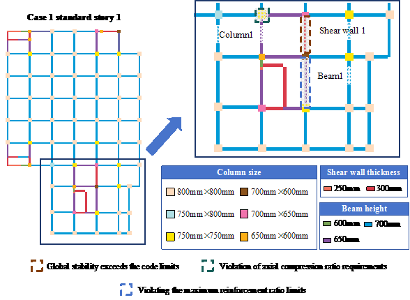
Figure 12. Representative components violating code requirements

Table 18. Summary of critical loads for non-compliant components

Component	Over-limit type	Verification contents	Value	Code limits
Column 1	Violation of axial compression ratio requirements	Axial compression ratio	1.00	0.90
Shear wall 1	Global stability exceeds the code limits	Axial force	35,480 kN	33,452 kN
Beam 1	Violating the maximum reinforcement ratio limits	Reinforcement ratio	2.90%	2.75%

As shown in Figure 12 and Table 18, a typical case analysis of non-compliant components is conducted based on component dimensions and applied loads, as follows:

(a) The majority of columns have a section of 800 mm × 800 mm, whereas the over-limit Column 1 has a significantly smaller section of 750 mm × 750 mm. Under combination loads, this column sustains a significant axial compressive force, causing the axial compression ratio to exceed the code-specified limit. This indicates that an insufficient section size is the primary cause of the axial compression ratio exceeding the limit.

(b) Both shear walls have a thickness of 300 mm. Shear wall 1 sustains even larger shear forces under the same seismic loading cases, but due to its relatively small size, its stability is significantly reduced, leading to a stability over-limit. This indicates that intelligent design methods inadequately address stability verification under complex loading conditions.

(c) The majority of beams have a height of 700 mm, while the over-reinforced Beam 1 has a notably smaller height of 650 mm. Under combined loads, the beam experiences a critical end moment and corresponding shear force, resulting in an over-reinforced condition with respect to the tension reinforcement ratio, indicating that insufficient beam height is the direct cause of the over-reinforcement.

Furthermore, a limited subset of members (below 5%) may violate specific code limits (such as those governing the shear-compression ratio, axial compression ratio, or maximum reinforcement ratio) necessitating manual intervention. Even when accounting for both data preprocessing and subsequent adjustments, the AI-assisted generative design completes the end-to-end member-sizing process in just 30 minutes. This represents an approximately fivefold efficiency gain compared to the 2 to 3 hours typically required for a fully manual process.

7. Conclusion and Limitations

Aiming at the inefficiency and high cost in designing frame shear wall structures for industrial parks, this research introduces an improved HGNN model incorporating the SE attention mechanism and PN normalization, enabling generative design of structural member sizes. The key conclusions are as follows:

(a) Data representation and dataset development: A heterogeneous graph dataset encoding detailed load information was built from 101 real industrial-park frame-shear wall structures. The dataset represents structural members as nodes and their connections as edges. An enhanced graph schema was introduced, which explicitly models shear wall end columns and extends their connectivity. Comparative experiments on heterogeneous graphs show that the proposed representation mode, which includes shear wall end columns and expanded shear wall connectivity, can better capture structural topological features, resulting in an MRE decrease of approximately 3% compared to conventional topological representations.

(b) Novel HGNN model training and test: To address the regression limitations of unimproved HGNNs on heterogeneous structural data, an improved HGNN was developed by integrating the Squeeze-and-Excitation (SE) attention mechanism with the PairNorm (PN) normalization module. Ablation studies and five-fold cross-validation demonstrate its effectiveness, achieving an average RMSE reduction of approximately 21% relative to the unimproved HGNN, with the reduction for column dimensions approaching 30%.

(c) Engineering case studies: The model's practical value has been validated across three independent cases. It achieves over 70% consistency with engineer-designed solutions and improves design efficiency by approximately fivefold. The structural design software PKPM verifies that the generated solutions generally meet the global structural control indices stipulated in Chinese seismic design codes. However, at the component level, local non-compliant members persist in all three cases, primarily involving axial compression ratio, global stability, and maximum reinforcement ratio limits. Approximately 95% of components are code-compliant without modification, while the remaining components require engineer-led local adjustments. Therefore, the proposed model should be regarded as an auxiliary tool for preliminary sizing design rather than a substitute for structural analysis, code-compliance verification, and professional engineering judgment.

This study also has certain limitations. First, the scale of the dataset used is relatively small, and future work should expand the current dataset. Meanwhile, a self-supervised heterogeneous graph representation learning strategy will be adopted to mitigate this limitation in future work. Furthermore, the generalization capability of the proposed improved HGNN model for complex scenarios, such as irregular structures and super-tall buildings, still requires further validation. Moreover, real-world industrial park structures often involve complex multi-way dependencies. Hypergraph neural networks ^[45] and cross-attention ^[46] mechanisms have shown promising capability in relational representation within heterogeneous graphs. In future work, we will further explore these directions to achieve more expressive relational representations.

Acknowledgments

This work was supported by the Beijing Municipal Natural Science Foundation (8252008), Sichuan Science and Technology Program (2025ZNSFSC1312), and Fundamental Research Funds for the Central Universities (2682025CX041, 202510613013), and Research Funds for the China Southwest Architecture Design & Research Inst Co., Ltd. (R-2025-84-S-Y-2027).

Data Availability Statement

The datasets and code generated during the current study are available from the corresponding author upon reasonable request.

References

[1]     H. Zhang, Construction technology of frame shear wall structure in construction engineering, Proceedings of the 2016 International Conference on Education, Management, Computer and Society, Atlantis Press, 2016, pp. 1443-1446. https://doi.org/10.2991/emcs-16.2016.361.

[2]     Y. Feng, Y. Fei, Y. Lin, W. Liao, X. Lu, Intelligent generative design for shear wall cross-sectional size using rule-embedded generative adversarial network, Journal of Structural Engineering, 149 (2023) 04023161. https://doi.org/10.1061/JSENDH.STENG-12206.

[3]     T.B. Nerenst, M. Ebro, M. Nielsen, T. Eifler, K.L. Nielsen, Exploring barriers for the use of FEA-based variation simulation in industrial development practice, Design Science, 7 (2021) e21. https://doi.org/10.1017/dsj.2021.21.

[4]     C. Perea, J. Alcala, V. Yepes, F. Gonzalez-Vidosa, A. Hospitaler, Design of reinforced concrete bridge frames by heuristic optimization, Advances in Engineering Software, 39 (2008) 676-688. https://doi.org/10.1016/j.advengsoft.2007.07.007.

[5]     H. Rostami Najafabadi, T.C. Martins, M.S.G. Tsuzuki, A. Barari, Structural design with self-weight and inertial loading using simulated annealing for non-gradient topology optimization, Machines, 12 (2024) 25. https://doi.org/10.3390/machines12010025.

[6]     M. Rostami, D. Moradinezhad, A. Soufipour, Improved and competitive algorithms for large scale multiple resource-constrained project-scheduling problems, KSCE Journal of Civil Engineering, 18 (2014) 1261-1269. https://doi.org/10.1007/s12205-014-0401-x.

[7]     P.K. Navin, Y.P. Mathur, Layout and component size optimization of sewer network using spanning tree and modified PSO algorithm, Water Resources Management, 30 (2016) 3627-3643. https://doi.org/10.1007/s11269-016-1378-7.

[8]     A. Kaveh, S. Rezazadeh Ardebili, An improved plasma generation optimization algorithm for optimal design of reinforced concrete frames under time-history loading, Structures, 34 (2021) 758-770. https://doi.org/10.1016/j.istruc.2021.08.040.

[9]     R. Bodalal, Combined size and shape optimization of truss structures using the heap-based optimizer (HBO) algorithm, Arabian Journal for Science and Engineering, 50 (2025) 12689-12716. https://doi.org/10.1007/s13369-024-09372-0.

[10]  T. Dede, Y. Ayvaz, Combined size and shape optimization of structures with a new meta-heuristic algorithm, Applied Soft Computing, 28 (2015) 250-258. https://doi.org/10.1016/j.asoc.2014.12.007.

[11]  M. Cosut, G. Bekdas, S.M. Nigdeli, U. Isikdag, Predicting design suitability of box-shaped sustainable timber structural members using machine learning and hyperparameter optimization, Neural Computing and Applications, 37 (2025) 24123-24148. https://doi.org/10.1007/s00521-025-11556-0.

[12]  W. Shan, J. Liu, J. Zhou, Integrated method for intelligent structural design of steel frames based on optimization and machine learning algorithm, Engineering Structures, 284 (2023) 115980. https://doi.org/10.1016/j.engstruct.2023.115980.

[13]  Y. Pan, L. Zhang, Roles of artificial intelligence in construction engineering and management: a critical review and future trends, Automation in Construction, 122 (2021) 103517. https://doi.org/10.1016/j.autcon.2020.103517.

[14]  N. Nauata, S. Hosseini, K.-H. Chang, H. Chu, C.-Y. Cheng, Y. Furukawa, House-GAN++: generative adversarial layout refinement network towards intelligent computational agent for professional architects, Proceedings of the IEEE/CVF Conference on Computer Vision and Pattern Recognition, 2021, pp. 13632-13641. https://doi.org/10.1109/CVPR46437.2021.01342.

[15]  W. Liao, X. Lu, Y. Huang, Z. Zheng, Y. Lin, Automated structural design of shear wall residential buildings using generative adversarial networks, Automation in Construction, 132 (2021) 103931. https://doi.org/10.1016/j.autcon.2021.103931.

[16]  Y. Gu, Y. Huang, W. Liao, X. Lu, Intelligent design of shear wall layout based on diffusion models, Computer-Aided Civil and Infrastructure Engineering, 39 (2024) 3610-3625. https://doi.org/10.1111/mice.13236.

[17]  B. Fu, Y. Gao, W. Wang, A physics-informed deep reinforcement learning framework for autonomous steel frame structure design, Computer-Aided Civil and Infrastructure Engineering, 39 (2024) 3125-3144. https://doi.org/10.1111/mice.13276.

[18]  S. Qin, Y. Fei, W. Liao, X. Lu, Leveraging data-driven artificial intelligence in optimization design for building structures: a review, Engineering Structures, 341 (2025) 120810. https://doi.org/10.1016/j.engstruct.2025.120810.

[19]  Y. Zhao, H. Li, H. Zhou, H.R. Attar, T. Pfaff, N. Li, A review of graph neural network applications in mechanics-related domains, Artificial Intelligence Review, 57 (2024) 315. https://doi.org/10.1007/s10462-024-10931-y.

[20]  F. Scarselli, M. Gori, A.C. Tsoi, M. Hagenbuchner, G. Monfardini, The graph neural network model, IEEE Transactions on Neural Networks, 20 (2009) 61-80. https://doi.org/10.1109/TNN.2008.2005605.

[21]  P. Zhao, W. Liao, Y. Huang, X. Lu, Intelligent design of shear wall layout based on graph neural networks, Advanced Engineering Informatics, 55 (2023) 101886. https://doi.org/10.1016/j.aei.2023.101886.

[22]  Y. Fei, S. Qin, W. Liao, H. Guan, X. Lu, Graph neural network-assisted evolutionary algorithm for rapid optimization design of shear wall structures, Advanced Engineering Informatics, 65 (2025) 103129. https://doi.org/10.1016/j.aei.2025.103129.

[23]  N. Nourian, M. El-Badry, M. Jamshidi, Design optimization of truss structures using a graph neural network-based surrogate model, Algorithms, 16 (2023) 380. https://doi.org/10.3390/a16080380.

[24]  M. Li, Y. Liu, B.C.L. Wong, V.J.L. Gan, J.C.P. Cheng, Automated structural design optimization of steel reinforcement using graph neural network and exploratory genetic algorithms, Automation in Construction, 146 (2023) 104677. https://doi.org/10.1016/j.autcon.2022.104677.

[25]  P. Zhao, Y. Fei, Y. Huang, Y. Feng, W. Liao, X. Lu, Design-condition-informed shear wall layout design based on graph neural networks, Advanced Engineering Informatics, 58 (2023) 102190. https://doi.org/10.1016/j.aei.2023.102190.

[26]  P. Ruan, W. Wen, C. Zhang, C. Zhai, Interior information inference and seismic response prediction of RC frames based on building contours and physics-enhanced graph neural network, Journal of Building Engineering, 112 (2025) 113921. https://doi.org/10.1016/j.jobe.2025.113921.

[27]  C. Zhang, D. Song, C. Huang, A. Swami, N.V. Chawla, Heterogeneous graph neural network, Proceedings of the 25th ACM SIGKDD International Conference on Knowledge Discovery & Data Mining, Association for Computing Machinery, Anchorage, AK, USA, 2019, pp. 793–803. https://doi.org/10.1145/3292500.3330961.

[28]  S. Qin, W. Liao, Y. Huang, S. Zhang, Y. Gu, J. Han, X. Lu, Intelligent design for component size generation in reinforced concrete frame structures using heterogeneous graph neural networks, Automation in Construction, 171 (2025) 105967. https://doi.org/10.1016/j.autcon.2025.105967.

[29]  Y. Li, C. Wang, S. Lv, W. Hou, StructureGraph: a universal performance evaluation method for engineering structures via heterogeneous graph neural network, Structural and Multidisciplinary Optimization, 68 (2025) 43. https://doi.org/10.1007/s00158-025-03969-1.

[30]  R. Tian, H. Sun, B. Mei, Y. Fu, W. Zhu, A heterogeneous graph neural network with spatial-temporal and operating condition-aware message passing mechanism for RUL prediction of aero-engines, Advanced Engineering Informatics, 73 (2026) 104507. https://doi.org/10.1016/j.aei.2026.104507.

[31]  M. Urbieta, M. Urbieta, T. Laborde, G. Villarreal, G. Rossi, Generating BIM model from structural and architectural plans using artificial intelligence, Journal of Building Engineering, 78 (2023) 107672. https://doi.org/10.1016/j.jobe.2023.107672.

[32]  J. Hou, C. Luo, F. Qin, Y. Shao, X. Chen, FuS-GCN: efficient B-rep based graph convolutional networks for 3D-CAD model classification and retrieval, Advanced Engineering Informatics, 56 (2023) 102008. https://doi.org/10.1016/j.aei.2023.102008.

[33]  X. Teng, M. Zhong, J. Liu, A self-supervised heterogeneous graph attention model based on adaptable step-size metapaths, IEEE Transactions on Neural Networks and Learning Systems, 36 (2025) 18020-18034. https://doi.org/10.1109/TNNLS.2025.3587020.

[34]  J. Su, L. Mao, C. Wu, BG-HGNN: toward efficient learning for complex heterogeneous graphs, arXiv preprint arXiv:2403.08207, 2024. https://doi.org/10.48550/arXiv.2403.08207.

[35]  J. Hu, L. Shen, G. Sun, Squeeze-and-excitation networks, IEEE Transactions on Pattern Analysis and Machine Intelligence, 42(8) (2020) 2011-2023. https://doi.org/10.1109/TPAMI.2019.2913372.

[36]  L. Zhao, L. Akoglu, Pairnorm: tackling oversmoothing in GNNs, ICLR 2020, 2019. https://doi.org/10.48550/arXiv.1909.12223.

[37]  R. Bing, G. Yuan, M. Zhu, F. Meng, H. Ma, S. Qiao, Heterogeneous graph neural networks analysis: a survey of techniques, evaluations and applications, Artificial Intelligence Review, 56 (2023) 8003-8042. https://doi.org/10.1007/s10462-022-10375-2.

[38]  S. Chaturvedi, T. Nagpal, V.S. Tiwari, Building structures 3-D modeling for indoor routing, 2022 International Conference on Futuristic Technologies (INCOFT), 2022, pp. 1-5. https://doi.org/10.1109/incoft55651.2022.10094367

[39]  Y. Yu, Y. Chen, W. Liao, Z. Wang, S. Zhang, Y. Kang, X. Lu, Intelligent generation and interpretability analysis of shear wall structure design by learning from multidimensional to high-dimensional features, Engineering Structures, 325 (2025) 119472. https://doi.org/10.1016/j.engstruct.2024.119472.

[40]  J. Ochshorn, Structural Elements for Architects and Builders, Butterworth-Heinemann (an imprint of Elsevier Press), 2010.

[41]  T.N. Kipf, M. Welling, Semi-supervised classification with graph convolutional networks, arXiv preprint arXiv:1611.07308, 2016. https://doi.org/10.48550/arXiv.1609.02907.

[42]  P. Veličković, G. Cucurull, A. Casanova, A. Romero, P. Lio, Y. Bengio, Graph attention networks, arXiv preprint arXiv:1710.10903, 2017. https://doi.org/10.48550/arXiv.1710.10903.

[43]  X. Wang, H. Ji, C. Shi, B. Wang, Y. Ye, P. Cui, P.S. Yu, Heterogeneous graph attention network, The World Wide Web Conference, Association for Computing Machinery, San Francisco, CA, USA, 2019, pp. 2022-2032. https://doi.org/10.1145/3308558.3313562.

[44]  Z. Hu, Y. Dong, K. Wang, Y. Sun, Heterogeneous graph transformer, Proceedings of The Web Conference 2020, Association for Computing Machinery, Taipei, China, 2020, pp. 2704-2710. https://doi.org/10.1145/3366423.3380027.

[45]  S. Mo, X. Teng, K. Wu, J. Liu, K. Yuan, A universal subhypergraph-assisted embedding framework for both homogeneous and heterogeneous networks, IEEE Transactions on Knowledge and Data Engineering, 37 (2025) 4935-4947. https://doi.org/10.1109/TKDE.2025.3581963.

[46]  D. Zhao, Y. Chen, W. Song, Q. He, Cross-view self-supervised heterogeneous graph representation learning, Neural Networks, 190 (2025) 107681. https://doi.org/10.1016/j.neunet.2025.107681.