1. Introduction

An increasing number of large-scale structural dynamic analyses have been performed recently [1每5]. The resulting data of these analyses are time-varying in different time steps. In addition, these analyses often result in dozens of gigabytes (GB) of data, which are massive for 3D visualization [6]. In the post-processor of general structural dynamic analysis software (e.g., MSC.Marc, ANSYS, ABAQUS) [7每9], the rendering process for massive time-varying data is exceedingly slow, sometimes in excess of one hour for large-scale analyses. To smoothly display the structural dynamic process, most structural analysis software transforms the results to pre-computed animations [7每9]. However, such animations cannot solve the fundamental rendering problems. Most of them merely display the dynamic process at a fixed viewing angle and position, and lack the necessary interactive operations. Consequently, high-speed rendering of such massive amount of time-varying data has become an important issue for large-scale structural dynamic analyses.

Although several methods for accelerating the rendering process of massive static data have been proposed [10每11], rendering time-varying data of large-scale structural dynamic analyses is a much more complicated task [12每13]. In the process of rendering, static data needs to be visited once only, whereas time-varying data requires continuous visit in order to display a dynamic process. Thus, time-varying data must be stored in a GPU memory for quick visit in the process of rendering. However, the GPU memory size is in general 1每2 GB, and at most 4 GB [14], therefore the massive amount of time-varying data cannot be completely stored in a GPU memory. In this case, these data need to be continuously transmitted from the host memory to the GPU memory during the rendering process. Such a data transmission is relatively slow compared to the direct access in the GPU memory, and most rendering time elapses during this data transmission [15]. These problems are the primary cause for an inefficient rendering of massive time-varying data, which presents a big challenge for high-speed visualization of large-scale structural dynamic analyses.

To minimize the issue of slow data transmission and achieve high-speed rendering, solutions to two key technical problems are necessary to be obtained: Solution 1 每 significantly reducing the size of time-varying data to satisfy the capacity limit of a GPU memory; and Solution 2 每 efficiently reconstructing a complete structural dynamic process in the process of rendering.

To obtain Solution 1, the key frame extraction method is considered appropriate for reducing massive time-varying data in a structural dynamic analysis. The time steps in such an analysis are referred to as the frames in visualization. Several techniques in relation to key frame extractions are proven to be suitable for identifying the representative time steps in dynamic analyses [16每23]. The extracted time steps are generally a small fraction of the total time steps, thereby significantly reducing the amount of massive time-varying data [20每23]. During the dynamic process, a structure may develop large non-linear deformations, leading to complicated 3D movements. Note that some existing extraction methods developed for 3D data are mainly targeted for motions of a limited number of predefined objects (e.g., some rigid-body motions) or points (e.g., motion capture data at some predefined points) [18每19]. As such they are unsuitable for simulating complicated 3D movements. On the other hand, the clustering method, as one of the widely used key frame extraction methods, has the advantage of handling complicated 3D movements [20每23], and is therefore well suited for structural dynamic analysis. In spite of this, the existing clustering method [20每23] was not originally designed for the GPU-based rendering and cannot be adapted to different GPU platforms, because the size of the extracted key frames may exceed the memory limitation of a GPU. In view of the above, a key frame extraction method specific to the GPU-based rendering is thus necessary to be developed.

To obtain Solution 2, a GPU-based frame interpolation is considered in this study. Note that 3D visualizations generated directly from the extracted key frames are not complete at all. Therefore, frame interpolation is necessary for reconstructing the entire dynamic process of the structures. Note also that due to the GPU hardware limitations in the past, early studies on GPU-based frame interpolations could not achieve satisfactory performance [24]. Since the 2006 release of GPUs with unified architecture, its computational performance and programming convenience have improved significantly [25]. Nevertheless, related studies [26每28] indicated that the access efficiency of data in a GPU memory has become an important bottleneck in the frame interpolation of time-varying data. This is because large amount of data must be continuously accessed from the GPU memory in the process of frame interpolation. It is worth noting that the GPU has a complicated memory system and any non-optimized access model may result in significant memory latency and unacceptable low efficiency. Therefore, a novel data access model is highly desirable for high-efficient GPU-based frame interpolation. Such a model should take a full consideration of the characteristics of time-varying data in structural dynamic analyses as well as the special features of the GPU memory system. Although high-speed 3D visualization in civil engineering and construction has been extensively studied [29每32], an efficient data access model has not yet been proposed.

A complete GPU-based solution for high-speed visualization of massive time-varying data in large-scale structural dynamic analyses is thus developed in this study. To address the issue of GPU memory limitations, a specialized key frame extraction algorithm based on the clustering concept is proposed that is adaptive to different GPU platforms and can significantly reduce the size of time-varying data. Using the key frames, a GPU-based parallel algorithm for frame interpolation is also proposed to reconstruct the complete structural dynamic process. Particularly, a novel data access model considering the features of time-varying data and GPU memory is designed to further improve the interpolation efficiency. Two case studies including a stone arch bridge and a high-rise building are investigated to demonstrate the advantages of the proposed solution.

2. Overall visualization framework

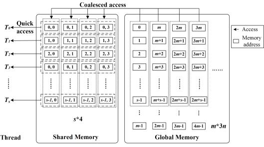
The overall framework of high-speed visualization of massive time-varying data resulted from a large-scale structural dynamic analysis is illustrated in Figure 1. In this framework, data transmission from the host memory to the GPU memory is implemented once only before rendering. Hence, instead of slow data transmission, key frame extraction and parallel frame interpolation will dominate the rendering efficiency for time-varying data visualization.

Three platforms are used for this framework: (1) a graphics platform, (2) a software development platform and, (3) a hardware platform. An open-source graphics engine, OSG (OpenSceneGraph), is adopted as the graphics platform to implement some in-depth visualization developments [33]. The CUDA (Compute Unified Device Architecture) platform, being the most widely used in general GPU computing development, is adopted as the software development platform [34]. Accordingly, a video card supporting CUDA, e.g., Quadro FX 3800 (192 cores, 1GB memory, widely used in desktop computers), is adopted as the hardware platform. The osgCompute library developed by the University of Siegen [35] is used to integrate OSG and CUDA. Using these platforms, the entire process of visualization can be fully controlled from software to hardware, which provides a convenient foundation for solving the visualization problems for massive time-varying data.

3. Clustering-based key frame extractions

The time-varying data of a structural dynamic analysis includes displacements, stresses, velocities, etc. Note that this study focuses on the nodal displacement data which are used as references for visualizing other types of data. The proposed extraction algorithm divides the entire process of movement into several sub-processes (i.e., clusters). Although sub-processes are quite different from each other, there is a significant similarity within each sub-process; thus a few key frames are adequate to represent the entire sub-process. The first, middle and last frames of each cluster are selected as the key frames, which correspond to the beginning, developing and finishing stages of the sub-processes, respectively.

The purpose of key frame extraction is to satisfy the constraints of a GPU memory, i.e., the total volume of key frames must be lower than that of a GPU memory. As mentioned above, a cluster can produce three key frames (two boundaries and one middle), however two adjacent clusters share the same boundary frame. Defining the number of clusters and that of key frames as N_c and k, respectively, we have k = 2N_c + 1. The number and volume of the total frames are defined as N_f and V_f, respectively. The variable V_v represents the volume of the GPU memory. Given that the data volume of the key frames kV_f / N_f should be smaller than V_v, the maximum of N_c can then be calculated by Eq. (1):

The larger N_c is, the larger k is, which implies that more key frames are produced for a more complete visualization. Theoretically,  should be aimed for. However, N_c does not reach  in reality because the GPU memory also stores other required data (e.g., structural model and textures), namely the static data which do not change with different time steps. The GPU memory size used for static data varies for different rendering problems and different GPU platforms, which can be measured by using some memory monitoring software (e.g., RivaTuner [36]). In this study, the value of N_c is approximately 0.8 for the case studies (presented in Section 5) and the specified hardware platform (see Section 2). In other cases (e.g., in which extreme large texture is required), however, an optimal value for N_c should be calculated based on the measurement using RivaTuner or other software with similar functions.

The coordinates of all graphical vertices in each frame are available from the structural dynamic analysis. In the i^th frame, the vector consisting of all vertices is defined as a frame vector, i.e., X_i. If the total number of vertices is n, the distances between two different frame vectors [37], i.e., X_i and X_j, can be calculated by Eq. (2):

where x_i,l, y_i,l and z_i,l are the 3D coordinates of the l^th vertex in the i^th frame.

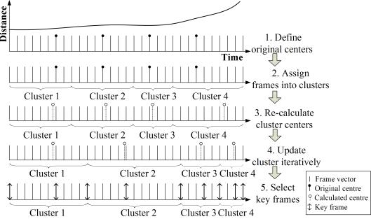
The distance calculated in Eq. (2), which represents the degree of movement of the structure between two frames, is selected as the criterion of clustering. Based on this criterion, the proposed key frame extraction algorithm is outlined as follows:

(1) Define the original cluster centers

N_c frame vectors, , j = 1, 2, ＃N_c, are extracted from the N frame vectors at the same time interval as the original cluster centers.

(2) Assign frames into clusters

Between the two adjacent clusters, a frame vector must be assigned to the cluster with the shorter distance to its center.

(3) Re-calculate cluster centers

After all frames are assigned to the corresponding clusters, the cluster centers are re-calculated according to Eq. (3):

where  is the number of frame vectors in the j^th cluster.  represents the calculated center of the j^th cluster. It is noted that  is a mean vector and is possibly not a real frame vector.

(4) Update the cluster iteratively

Repeat Steps (2) 每 (4) until all the cluster centers, , do not alter any more.

(5) Select key frames

For each cluster, the boundary frames and the frame that is the closest to the cluster center  are selected as the key frames.

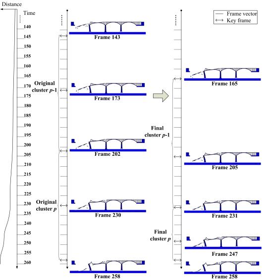
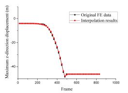
The above process of extracting key frames is illustrated in Figure 2. The horizontal axis refers to a time scale, whereas the vertical axis represents the distances of different frame vectors. Thus, the curve in Figure 2 describes the change in distances. The larger the slope of this curve, the more significant the movements are. Figure 2 shows that more key frames are extracted for significant changing phases, and vice versa, which can better demonstrate the characteristics of a structural dynamic process.

4. Parallel frame interpolation

4.1 Interpolation model based on the B-spline

The spline-based interpolation, one of the most important interpolation methods, has been widely used in such fields as computer graphics, structural analysis and 3D modeling [38每39]. Comparison of the three popular splines (i.e., Bezier spline, B-spline and NURBS [40]) indicates that, Bezier spline is too sensitive to local errors and NURBS is too complicated and computationally inefficient. The cubic uniform B-spline is considered appropriate for this study, because it can rationally simulate the complicated movement curves with high computational performance.

There are k 每 1 time intervals in the total k key frames. For the j^th vertex at the i^th time interval, the interpolation equation  representing the movement curve is presented in Eq. (4), based on the cubic uniform B-spline:

where u is the variable of this curve. The parameters V_{i, j} to V_{i+3, j} are the control points for the interpolation of the j^th vertex at the i^th time interval.

According to the key frame data, the control points of the j^th vertex for the k 每 1 time intervals can be solved by Eq. (5):

where Q_{i, j}, for i = 0, 1, ＃, k 每 1, represents the coordinates of the j^th vertex for different key frames.

After the control points are determined, the interpolation of the j^th vertex can be performed using Eq. (4). It should be noted that the above interpolation must be performed repeatedly for numerous vertices in an entire structure. Thus, high-performance GPU computing is necessary for such repetitive frame interpolation.

4.2 GPU-based parallel frame interpolation

To improve the computational efficiency, frame interpolation must make a full utilization of the parallel performance of a GPU. Note that there are a large number of vertices in a structural dynamic analysis. Every vertex has three coordinate components, and each component uses a thread to implement the interpolation process. This results in a massive number of threads, which are beneficial to maximize the potential of parallel performance of a GPU in CUDA [41].

Based on the above strategy, the parallel algorithm for frame interpolation is outlined as follows:

1) Set up the thread structure

The structure of CUDA has three levels, i.e., grid, block and thread [41]. The structure of the threads is determined by grids and blocks. Given that the graphical vertices are stored in a single-dimensional array, grids and blocks are also organized in a single-dimensional form. Due to hardware demands, the number of threads in one block must be an integer multiple of 32 but no more than 512. For most cases, 256 threads in a block are considered suitable [41]. In this study, the variable n represents the number of vertices and the total number of threads is 3n, which is equal to the number of vertex coordinate components. Therefore the total number of blocks should be 3n/256 or 3n/256+1, depending on whether 3n can be divided exactly by 256. As such, the running threads can simulate all the vertex coordinate components.

2) Define the variables

The interpolation requires three types of data: the graphical vertices, an interpolation parameter u and the control points V_i. The graphical vertices, named vertices, are a single-dimensional array stored in the GPU memory and are updated dynamically in the process of interpolation. The parameter u is a float parameter ranging from 0 to 1 and can be determined by the current interpolation frame and the corresponding four adjacent key frames. The control points V_i are stored in a 2D float array located in the Shared Memory of GPU, namely s_data [256][4], which is specially designed to improve the access efficiency (as discussed in Section 4.3).

3) Execute the interpolation

In each interpolation, a coordinate component is interpolated by one thread. Except for the thread IDs, the executing codes based on Eq. (4) are identical for all the threads, as follows:

vertices[vertIdx] = 1.0/6.0*( (1每3*u+3*u*u每u*u*u)*s_data[threadIdx.x][0]

+ (4每6*u*u+3*u*u*u)* s_data[threadIdx.x][1]

+ (1+3*u+3*u*u每3*u*u*u)* s_data[threadIdx.x][2]

+ (u*u*u)* s_data[threadIdx.x][3] );

where vertIdx is the global ID of the thread and is used to calculate the corresponding graphical vertices. threadIdx.x is the local ID inside the block and is used to access the control points stored in the Shared Memory which can only be shared inside a block.

The complete frame interpolation includes three steps: interpolation, mapping and rendering, as illustrated in Figure 3. Interpolation is performed first which provides the vertices movement data. Mapping is an intermediate step for displaying the interpolation results by CUDA. Being a general numerical computing platform, CUDA has no direct relation to graphics rendering. Thus, the interpolation results are mapped to OSG as vertex buffer objects (VBOs) using the function map() of osgCompute [35], which is a very convenient way to implement the mapping operation. The rendering step transforms VBOs to pixels on the OSG platform and displays the results of frame interpolation. The above three steps, as seen in Figure 3, forms a seamless process in which the interpolation calculation and rendering are integrated.

4.3 Optimized access model based on the Shared Memory

A GPU has six types of memory (e.g., Global Memory, Shared Memory and Texture Memory), which vary significantly in capacity and speed [42]. Although data access in a GPU memory is faster than that between the host memory and the GPU memory, any non-optimized access model may result in low interpolation efficiency due to the complicated memory system of a GPU.

The Global Memory is the main platform for data exchange between GPU and host. However, it has a great access latency for approximately 400每600 clock cycles. Coalesced access is an important method for reducing the access latency of the Global Memory [41]. When the data addresses are sequential and the size of each data is 4 bytes, 8 bytes or 16 bytes, the memory accesses of 16 adjacent threads are coalesced into one. Otherwise, each thread accesses the Global Memory individually, resulting in a much lower access speed.

In frame interpolation, the control points V_i are the largest dataset amongst all data and their access speed is a major bottleneck to the interpolation efficiency. The coordinate components are stored in a single-dimensional float array. Thus, each component is 4 bytes, which satisfies one of the two coalesced access conditions. During the process of interpolation, each vertical component requires four corresponding control point components which however are not sequential in the Global Memory. As Figure 4 illustrates, when the number of control points is m, there are m address intervals between the memory addresses accessed by the two adjacent threads. Thus, the coalesced access cannot be satisfied in such component data structures.

The optimized data access model based on the Shared Memory is illustrated in Figure 5. The Shared Memory is a high-speed cache shared by all the threads in one block [41]. When a block has s threads (s = 256 in this study), a s℅4 array is created in the Shared Memory to store the four components of the control points for each thread, using the CUDA statement as __shared__ float s_data[s][4]. In this data access model, each row of s_data can access the Global Memory in a coalesced manner because of the sequential distribution of the control point components in the Shared Memory. After all the data in s_data are copied, each thread in a block can rapidly access the corresponding four control point components in the Shared Memory. This optimized model uses the Shared Memory as a data transferring platform to achieve the coalesced access for the Global Memory, which further improves the efficiency of interpolation.

5. High-speed visualization 每 case studies

5.1 High-fidelity collapse analysis of a stone arch bridge

A high-fidelity collapse analysis is presented for a four 65-m span highway stone arch bridge that was 328.54 m in length, 13 m in width, and 42min height [2]. The finite element (FE) model of this bridge has a total of 60,320 elements and 83,846 nodes, as illustrated in Figure 6. The analysis was performed by FE software MSC.Marc and produces approximately 12 GB of displacement data with a total of 832 time steps [2]. A video card with 1 GB memory (Quadro FX 3800) is employed to display the results. Therefore, the key frame extraction method is necessary to be adopted to satisfy the requirement of the GPU memory limitation.

A total of 56 key frames are extracted from the 832 time steps, and the total size of the key frames is 816 MB, smaller than the capacity of the GPU memory. The number of key frames is only 6.7% of the total number of frames, which indicates that the proposed extraction algorithm can reduce the data size significantly.

The extracted key frames can represent the typical characteristics of a structural dynamic process. Figure 7 compares the key frames in the original clusters with those in the final clusters in the range of 120 frames. In the original clusters, key frames are distributed uniformly with time. However, the structural movements become more significant towards the end of the collapse process due to gravitational acceleration and collision of the collapsed structural components with the ground. Hence, a more dense distribution of the key frames is required to better represent the end of the structural movement. In the final clusters, the selected key frames are sparse for the insignificant changing phase and dense near the end, as illustrated in Figure 7. Figure 8 presents the extracted key frames corresponding to the cluster boundaries. These typical key frames provide an important foundation for a satisfactory frame interpolation. It is evident that the key frames are able to exactly replicate the final stage of collapse for each span of the bridge, when the main arches collide with the ground. It should be noted that textures are used for a more realistic visualization.

The proposed GPU-based parallel frame interpolation is also performed. Figure 9 compares the interpolation results against the FE analysis outcomes [2] with a good agreement. To further validate the accuracy of frame interpolation, two comparisons of the typical movement curves between the interpolation results and the original FE data are demonstrated in Figure 10. The main arches are the most important bridge components and the direction z represents the main movement direction. A total of 50 points which are distributed uniformly in the main arches along the y-axis (see Figure 6) are selected, and their mean and maximum displacements in the z-direction are compared. The similarity coefficients between the interpolation results and original data are 0.9999 and 0.9997, respectively, for the mean and maximum displacements. This confirms that the accuracy of the proposed method is acceptable for reconstructing a structural dynamic process.

Based on the parallel interpolation algorithm, the interpolation time of all the vertices (83,846 vertices and 251,538 coordinate components) is only 0.0047 s per frame. Using the optimized data access model, the interpolation can be further improved to 0.0018 s per frame with a speedup ratio of 2.6, which fully satisfies the demands of high-speed rendering.

When the stone arch bridge is visualized in MSC.Marc, the time required for rendering a time step is approximately 3 s, and the entire rendering process (832 time steps) amounts to 42 min. When the same bridge is visualized by the proposed method, the rendering efficiency reaches 20 frames/s (i.e., 0.05 s per time step) and the entire rendering process requires only 41.6 s, almost 67 times improvement. This comparison further confirms that the proposed GPU-based method can achieve high-performance visualization for a large-scale structural dynamic analysis.

Furthermore, the synchronized walkthrough is also implemented in the bridge collapse visualization due to its high rendering efficiency, as shown in Figure 11; this offers a convenient way to fully observe the bridge collapse process. In this regard, the proposed method also provides an enhanced interactive visualization environment for large-scale structural dynamic analyses.

5.2 Dynamic analysis of a super high-rise building

A dynamic analysis is performed by MSC.Marc for a super high-rise building subjected to extremely strong earthquakes [3]. This building contains 124 stories with a total height of 632 m and adopts a hybrid lateral-force-resisting system referred to as ※mega-column/core-tube/outrigger§. Its FE model contains a total of 86,563 elements and 54,542 nodes. The analysis produces approximately 20 GB of time-varying data with total 2001 time steps.

Given the limitation of 1 GB GPU memory (Quadro FX 3800), the whole dynamic process is divided into 42 clusters and 86 key frames (832 MB) are selected by using the proposed algorithm. As a result, the extracted key frames are only 4.3% of the total time-varying data, which confirms that the proposed algorithm exhibits a high efficiency in data extraction.

To reconstruct the complete dynamic process, the GPU-based frame interpolation is performed using the extracted key frames. A good comparison between the original FE analysis data [3] and the interpolation results is achieved, as illustrated in Figure 12. Further, the top displacement of this building is also compared in Figure 13. The similarity coefficient between the two sets of results is found to be 0.9996, which again validates the rationality of the proposed frame interpolation method.

The optimized data access model plays an important role in improving the interpolation efficiency, by which the time for one interpolation of all vertices (54,542 vertices and 163,626 coordinate components) ranges from 0.0032 s to 0.0016 s, with a speedup ratio of 2.0. The larger the amount of data is, the more significant the advantage of the optimized access model is. As far as the speedup ratio is concerned, this case study has fewer vertices than the former one; hence a slightly lower speedup ratio is obtained. Nevertheless, such interpolation efficiency is adequate to satisfy the demands of high-speed rendering.

Using MSC.Marc, the rendering time is approximately 2 s for a time step in the analysis of the same high-rise building, and the entire rendering process (2001 time steps) takes one hour. Using the proposed method, on the other hand, the rendering efficiency reaches 30 FPS and the entire rendering process requires only 66.7 s; this is equivalent to 0.03 s per time step and also approximately 67 times improvement. Such an improvement once again confirms that high-performance visualization can be successfully achieved by the proposed method for a large-scale structural dynamic analysis.

6. Conclusion

A key frame extraction algorithm based on clustering concept is proposed to significantly reduce the data size to satisfy the requirement of GPU memory limitations. Superior to the relevant existing studies, the proposed algorithm is specific to GPU-based rendering and adaptive to different GPU platforms. Furthermore, the extracted key frames can satisfactorily represent typical characteristics of a structural dynamic process.

A GPU-based parallel frame interpolation algorithm is also proposed for large-scale structural dynamic analyses with high efficiency. Particularly, a novel data access model is developed taking into account the special features of time-varying data and GPU memory. Two case studies on a stone arch bridge and a high-rise building reveal that, by the proposed algorithm, an approximately 67 times improvement in rendering efficiency is achieved and the structural dynamic processes can be satisfactorily and reliably reconstructed.

Based on the proposed two algorithms, a complete solution to the traditionally inefficient rendering problems for massive time-varying datasets is presented, which provides a high-speed and interactive visualization environment for large-scale structural dynamic analyses.

Acknowledgements

The authors are grateful for the financial support received from ....

Reference

[1] M.V. Sivaselvan, O. Lavan, G.F. Dargush, H. Kurino, Y. Hyodo, R. Fukuda, et al., Numerical collapse simulation of large-scale structural systems using an optimization-based algorithm, Earthquake Engineering & Structural Dynamics 38 (5) (2009) 655每677.

[2] Z. Xu, X.Z. Lu, H. Guan, X. Lu, A.Z. Ren, Progressive-collapse simulation and critical region identification of a stone arch bridge, Journal of Performance of Constructed Facilities (ASCE) 27 (1) (2013) 43每52.

[3] X. Lu, X.Z. Lu, W.K. Zhang, L.P. Ye, Collapse simulation of a super high-rise building subjected to extremely strong earthquakes, Science China Technological Sciences 54 (10) (2011) 2549每2560.

[4] X.Z. Lu, X. Lu, H. Guan, W.K. Zhang, L.P. Ye, Earthquake-induced collapse simulation of a super-tall mega-braced frame-core tube building, Journal of Constructional Steel Research 82 (2013) 59每71.

[5] M. Hori, T. Ichimura, Current state of integrated earthquake simulation for earthquake hazard and disaster, Journal of Seismology 12 (2) (2008) 307每321.

[6] MSC Software, Marc 2013 User's Guide, MSC Software, Santa Ana, CA, USA, 2013.

[7] ANSYS Inc., ANSYS Workbench User's Guide, ANSYS Inc., Canonsburg, PA, USA, 2013.

[8] ABAQUS, Abaqus/CAE User's Manual, Dassault Syst豕mes, Providence, RI, USA, 2013.

[9] C. Johnson, Top scientific visualization research problems, Computer Graphics and Applications (IEEE) 24 (4) (2004) 13每17.

[10] A. Dietrich, E. Gobbetti, S.E. Yoon, Massive-model rendering techniques: a tutorial, Computer Graphics and Applications (IEEE) 27 (6) (2007) 20每34.

[11] E. Gobbetti, D. Kasik, S. Yoon, Technical strategies for massive model visualization, Proc., 2008 ACM symposium on Solid and physical modeling, ACM, New York, NY, 2008, pp. 405每415.

[12] C. Hansen, C.R. Johnson, The Visualization Handbook, Academic Press, Waltham, MA, USA, 2004.

[13] NVIDIA Corporation, NVIDIA products and technologies, http://www.nvidia.com/page/products.html 2013.

[14] M. Gokhale, J. Cohen, A. Yoo, W.M. Miller, A. Jacob, C. Ulmer, Hardware technologies for high-performance data-intensive computing, Computer 41 (4) (2008) 60每68.

[15] G.J. Sullivan, T. Wiegand, Video compression 每 from concepts to the H.264/AVC standard, Proceedings of the IEEE 93 (1) (2005) 18每31.

[16] C. Gianluigi, S. Raimondo, An innovative algorithm for key frame extraction in video summarization, Journal of Real-Time Image Processing 1 (1) (2006) 69每88.

[17] J. Calic, E. Izuierdo, Efficient key-frame extraction and video analysis, Proc., International Conference on Information Technology: Coding and Computing, IEEE Computer Society, Washington, DC, USA, 2002, pp. 28每33.

[18] K.S. Huang, C.F. Chang, Y.Y. Hsu, S.N Yang, Key probe: a technique for animation keyframe extraction, The Visual Computer 21 (8每10) (2005) 532每541.

[19] J. Xiao, Y. Zhuang, T. Yang, F. Wu, An efficient keyframe extraction from motion capture data, Advances in Computer Graphics 4035 (2006) 494每501.

[20] Y. Zhuang, Y. Rui, T.S. Huang, S. Mehrotra, Adaptive key frame extraction using unsupervised clustering, Proc., International Conference on Image Processing, IEEE Computer Society, Washington, DC, USA, 1998, pp. 866每870.

[21] S.P. Yang, X.G. Lin. Key frame extraction using unsupervised clustering based on a statistical model, Tsinghua Science & Technology 10 (2) (2005) 169每173.

[22] P. Mundur, Y. Rao, Y. Yesha, Keyframe-based video summarization using Delaunay clustering, International Journal on Digital Libraries 6 (2) (2006) 219每232.

[23] X. Zeng, W. Li, X. Zhang, B. Xu, Key-frame extraction using dominant-set clustering, 2008 IEEE International Conference on Multimedia and Expo, IEEE Computer Society, Washington, DC, USA, 2008, pp. 1285每1288.

[24] F. Kelly, A. Kokaram, Fast image interpolation for motion estimation using graphics hardware, SPIE Proceedings 5297 (2004) 184每194.

[25] D Kirk, NVIDIA CUDA software and GPU parallel computing architecture, Proc., 6th International Symposium on Memory Management, ACM, New York, NY, USA, 2007, pp. 103每104.

[26] D. Nagayasu, F. Ino, K. Hagihara, A decompression pipeline for accelerating out-of-core volume rendering of time-varying data, Computers & Graphics 32 (3) (2008) 350每362.

[27] M. Smelyanskiy, D. Holmes, J. Chhugani, A. Larson, D.M. Carmean, D. Hanson, et al., Mapping high-fidelity volume rendering for medical imaging to CPU, GPU and many-core architectures, IEEE Transactions on Visualization and Computer Graphics 15 (6) (2009) 1563每1570.

[28] J. Mensmann, T. Ropinski, K. Hinrichs, A gpu-supported lossless compression scheme for rendering time-varying volume data, Proc., 8th IEEE/EG International Conference on Volume Graphics, Eurographics Association Aire-la-Ville, Switzerland, 2010, pp. 109每116.

[29] T. Cheng, J. Teizer, Real-time resource location data collection and visualization technology for construction safety and activity monitoring applications, Automation in Construction 34 (2013) 3每15.

[30] C.Y. Chiu, A.D. Russell, Design of a construction management data visualization environment: A top每down approach, Automation in Construction 20 (4) (2011) 399每417.

[31] G. Esch; M.H. Scott, E. Zhang, Graphical 3D visualization of highway bridge ratings, Journal of Computing in Civil Engineering (ASCE) 23 (6) (2009) 355每362.

[32] Z. Xu, X.Z. Lu, H. Guan, A.Z. Ren, Physics engine-driven visualization of deactivated elements and its application in bridge collapse simulation. Automation in Construction 35 (2013) 472每481.

[33] D. Burns, R. Osfield, Open Scene Graph A: Introduction, B: Examples and Applications. Proc., IEEE Virtual Reality 2004, IEEE Computer Society, Washington, DC, USA, 2004, pp. 265.

[34] R. Farber, CUDA Application Design and Development, Morgan Kaufmann, San Francisco, CA, USA, 2011.

[35] University of Siegen, osgCompute documentation. http://www.basementmaik.com/doc/osgcompute/html/index.html 2012.

[36] Guru3D, RivaTuner. http://www.guru3d.com/content_page/rivatuner.html 2013.

[37] A.K. Jain, Data clustering: 50 years beyond K-means, Pattern Recognition Letters 31 (8) (2010) 651每666.

[38] T.M. Lehmann, C. Gonner, K. Spitzer, Addendum: B-spline interpolation in medical image processing, IEEE Transactions on Medical Imaging 20 (7) (2001) 660每665.

[39] S. Forstmann, J. Ohya , A. Krohn-Grimberghe, R. McDougall, Deformation styles for spline-based skeletal animation, Proc., 2007 ACM SIGGRAPH/Eurographics Symposium on Computer Animation, Eurographics Association Aire-la-Ville, Switzerland, 2007, pp. 141每150.

[40] G. Wahba, Spline Models for Observational Data, Society for Industrial and Applied Mathematics, Philadelphia, Pennsylvania, 1990.

[41] NVIDIA Corporation. NVIDIA CUDA C Programming Guide (Version 5.0). Santa Clara, USA, 2013.

[42] J. Sanders, E. Kandrot, CUDA By Example: An Introduction to General-Purpose GPU Programming, Addison-Wesley, Boston, MA, USA, 2010.