Notation list

l–The length of the Basic Grid;

w–The width of Basic Grid;

h–The height of the Basic Grid;

–The maximum number of the allowable Actors;

–The total number of fragments;

–The minimum number of fragments that are required to be simulated by one Actor;

–The average distance between the adjacent fragments;

–The distances between the ith fragment and the jth fragment;

–The number of generated fragments at the current time step;

–The minimum height of the Basic Grid to meet the demands of rendering efficiency;

–The minimum height of the Basic Grid to meet the demands of accuracy;

–The maximum height of the Basic Grid to meet the demands of accuracy;

–A calculation variable used during the iteration of height h;

–The normalized matrix of relative distance in z-axis;

–The sum of the ith row in ;

–A control variable in the clustering algorithm;

p–The central point of a fragment at the final time step using the clustering algorithm;

p*–The central point of a fragment at the final time step without fragment clustering algorithm;

–The error tolerance for evaluation of the accuracy of fragment simulations;

N*–The number of fragments for which .

1. Introduction

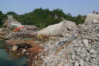
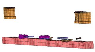
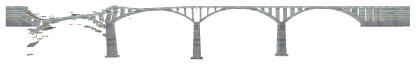
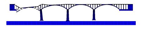
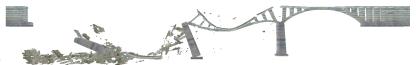
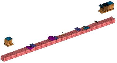
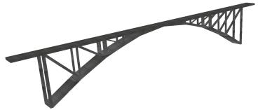
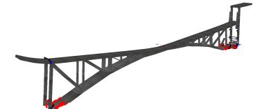
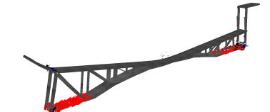
Bridges are very important lifeline infrastructures and bridge collapse events often cause many casualties and severe property losses [1–3]. Finite element (FE) analysis can accurately simulate the dynamic process of bridge collapses, and has therefore become one of the most popular numerical simulation methods used for detailed investigations of bridge collapse accidents [3–7]. Many FE studies indicate that “elemental deactivation” is one of the most suitable methods for collapse simulation [8–14]. To simulate the complicated nonlinear process of a structural collapse, elements that reach a certain level of damage are “deactivated” from the FE model and no longer participate in the subsequent calculation. However, due to the use of “elemental deactivation” technique, the results obtained directly from an FE analysis of a bridge collapse are usually incomplete and lack debris details. For example, a typical real bridge collapse accident is depicted in Figure 1, with the corresponding FE simulation results shown in Figure 2 [15]. A visual comparison of the two figures shows that large amount of fragments (deactivated elements) are not present in the FE analysis outcomes. Often in the investigation of a bridge collapse, debris comparisons are very important for determining whether the analysis results agree with the real situation, which will in turn contribute to the identification of the main reasons of a bridge collapse. As a consequence, the lack of representation of deactivated elements in the FE results precludes a direct comparison with the real accident.

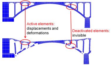
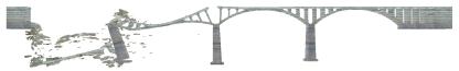
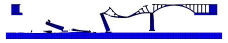
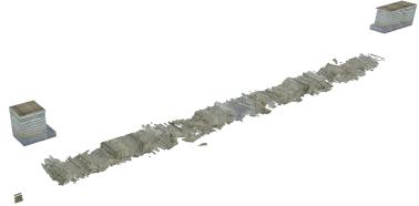
In current literatures, methods for visualizing deactivated elements have not yet been extensively studied. Deactivated elements are made invisible as reported in the published research [8–14] and in many general FE codes, such as ANSYS, ABAQUS, and MSC.Marc [16–18]. In an FE analysis of a bridge collapse, the active elements (i.e., the elements that are not deactivated) undergoing displacements and deformations are displayed in a graphical form; however once an element is deactivated, it becomes invisible in the post-process of the FE results, as indicated in Figure 3. In particular, when the bridge structural components collapse to the ground, a large number of elements are deactivated and become invisible. This explains why in Figure 2 a large amount of bridge debris is absent. Furthermore, the deactivated elements also make the collapse simulation less realistic and reliable (e.g., some elements disappear abruptly), which creates difficulties for non-professionals to fully understand the collapse situation based on the FE analysis outcomes. As described above, visualization of deactivated elements is a very challenging problem that demands better solutions for conducting detailed and reliable investigations of accidental bridge collapses.

Theoretically, the deactivated elements, representing the failed elements, are severely damaged and become fragments in the process of a bridge collapse. Fragment simulation techniques can therefore be adopted to visualize the deactivated elements. Such techniques can be classified into two categories according to their different rendering time: off-line simulation and real-time simulation [19]. The off-line simulation, often used for special movie effects, can produce high-fidelity fragment effects at the expense of long rendering time and costly computer hardware. On the other hand, the real-time simulation is highly efficient in producing fragment animations with good reality and powerful interactive functions. For this reason, the real-time simulation is widely used in 3D game productions. For a bridge collapse accident, repeated simulation is often necessary to help identify the most likely reasons of a collapse. This requires a high rendering efficiency which cannot be satisfied by the time-consuming off-line simulation; therefore the real-time simulation is a suitable alternative. In addition, the real-time simulation can also offer interactive operations for more convenient observations of a bridge collapse.

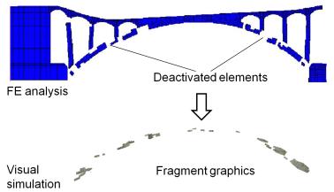
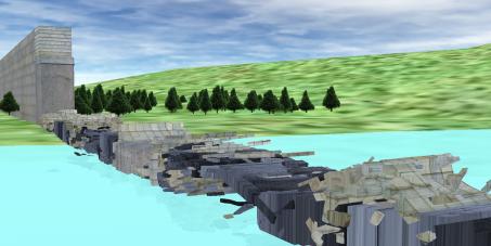
The process of fragment simulation constitutes of two stages: fragment generation and fragment movement. A number of simulation methods, such as physically based and geometrically based methods [20–24], have been proposed for fragment generation. Note that in the collapse simulation presented in this study, a considerably fine element mesh is made which can represent the size of the fragments. Note also that the generation of deactivated elements is based on an FE analysis and additional calculation is not required. Therefore, the fragments can be transformed directly from the deactivated elements. Specifically, once an element is deactivated in the FE analysis, a new graphical object of fragment is subsequently generated with the same shape and location as the corresponding deactivated element (Figure 4). This makes the fragment generation process very simple in concept and efficient in application.

The motion of fragments determines the distribution of bridge debris, which is a very important piece of information for bridge accident investigations. However, due to the absence of the deactivated elements in the FE computation, the simulation of fragment movement cannot be supported by the FE analysis results. To guarantee the reliability of the simulated fragment distribution, the fundamental laws of motion must be conformed, i.e. the simulated fragments undergo gravitational movement, and collide with the ground and structural components. A separate and accurate numerical calculation is thus necessary for such a simulation, which must also be efficient for a real-time simulation due to the large number of fragments being generated during a bridge collapse. Physics engines are considered an appropriate technique for fragment simulations [25]. They are specially designed computer codes and are employed to efficiently calculate the complicated physical behavior of moving bodies [26], such as smoke movement, water flow, rigid body dynamics, etc. In visual simulation, fragment movements are well featured by rigid body motion and collision, which happen to be the most remarkable simulation function of a physics engine. This makes the physics engine-driven visualization of deactivated elements more accurate and efficient.

In this paper, a 3D simulation method of fragment is proposed to visualize the deactivated elements, through an integration of a graphics engine, an FE analysis and a physics engine. To achieve a high rendering efficiency, a fragment modeling method is specially developed based on a grid-clustering algorithm. Using the proposed 3D visual simulation methodology, a complete, real-time and realistic process of collapse is reproduced, which provides necessary technical support for detailed investigations of bridge collapse accidents. A stone bridge and a reinforced concrete (RC) bridge are chosen as case studies to demonstrate the performance of the proposed visualization and simulation techniques.

2. Proposed simulation approach

The proposed integrated approach for fragment simulation is displayed in Figure 5, which consists of three major functional components: the FE analysis domain, the graphics engine domain and the physics engine domain. The graphics engine domain is a core component for implementing collapse visualization, while the FE domain and the physics engine domain provide necessary information for 3D visual simulation. During the process of simulation, the deformations and displacements of active elements are supported by the FE analysis, whereas the movements of the fragments transformed from the deactivated elements are determined by the physics engine, following the initial positions and shapes of the corresponding deactivated elements. The three domains must perform interactively as an integrated system, to ensure a realistic and smooth display of the bridge collapse process.

The above approach provides a prototype model to simulate and display the movement of the fragments. However, for the prototype model to be applicable to the practical cases, two critical problems are necessary to be solved.

(1) Amongst the aforementioned three domains, integration of the FE analysis and the graphics engine has been studied extensively [27–29]. However, integration of the three domains including the physics engine has not been reported in the existing literature. The development of an integrated simulation system is thus the primary aim of this study.

(2) The number of deactivated elements is extensively large in the FE analysis of a collapse. Despite the high efficiency of the physics engine, it is still a challenging task to perform complicated real-time calculation of the motion of a large number of fragments. Thus, a special algorithm for fragment dynamics simulation must be proposed with an improved efficiency.

3. Integrated simulation system

A graphics engine that offers a convenient user development privileges is an important foundation for achieving an integration of the three domains. In this study, an open-source graphics engine, i.e. OpenSceneGraph (OSG) [30], is adopted to implement in-depth modifications to meet the needs of the current development. As far as the physics engines are concerned, a comparison of the three popular physics engines, Havok, PhysX and Bullet [31–33], indicate that PhysX is most suitable for large scale numerical calculation of this study, because it adopts a multi-core GPU to accelerate computation [33]. Therefore, PhysX is adopted in this study to perform the numerical calculation of fragments.

To simulate a bridge collapse visually, the FE analysis and OSG are combined to display the displacements and deformations of the active elements. In this study, such a combination relies on the Callback mechanism of OSG [30], which implements the user requirement before rendering in each visualization frame. Using the Callback mechanism, the vertex coordinate vectors of the active elements are updated directly from the nodal displacements of the corresponding time steps. The entire updating process forms the animation of element displacements and deformations. More specifically, this updating process can be achieved by reloading UpdateCallback, a control class of the Callback mechanism [30]. The combined method of FE analysis and OSG is in general simple and straightforward. It can therefore be used to efficiently simulate the displacements and deformations of active elements during a bridge collapse.

To date, limited research has been reported on the integration between the two independent computer codes OSG and PhysX [34], due to their complicated application principles. Detailed discussions that follow not only demonstrate the proposed simulation technique but also provide a reference for other similar applications using OSG and PhysX. In this study, the Callback mechanism can also be used for fragment movement animation with the integrated OSG and PhysX. Specifically, the fragment vertex coordinates can be continuously updated in each frame using the real-time computing data of PhysX, which subsequently generates a fragment movement animation. For an accurate and smooth animation, two key steps are required for the OSG and PhysX integration: (1) establish a correlation between the fragment graphics of OSG and the dynamic bodies of PhysX, and (2) update the fragment graphics of OSG in each frame dynamically by the real-time data of PhysX.

A specific class, Fragments, is designed to establish the correlation between OSG and PhysX. In OSG, all the graphics are stored and managed by the class Geode [30]. The fragment graphics can also be created in Geode. While in PhysX, the class Actor is the fundamental computing unit, representing all the objects governed by the physical principles [33]. As such, a fragment in the class Fragments can be represented by both Geode and Actor, and a correlation between Actor and Geode can also be established. The initial parameters of Actor such as the initial position and shape are determined by Geode, thereby ensuring that the calculation requirements of PhysX are in accordance with the graphical display of OSG.

During fragment simulation, graphical display and physical computing are performed in parallel, which requires a dynamic link. This leads to a new class, Move-callback, which is designed to update the fragment graphics in each frame by the real-time data of PhysX. Inheriting the control class of Callback mechanism, Move-callback is able to control the major loop of fragment rendering (see Figure 6). In every frame, Move-callback obtains the movement information from Actors in PhysX, and such information is subsequently used to update the fragment graphics. This looping process forms animation of the fragments, as illustrated in Figure 6.

An efficient and integrated OSG and PhysX platform is thus established, based on the class Fragments and the class Move-callback, to achieve a real-time simulation of fragments. More importantly, independent features of PhysX and OSG are maintained in relation to their modeling processes. This helps to lay a solid foundation for solving the subsequent rendering problems in fragment simulation.

4. Fragment modeling

During the process of a bridge collapse, extensive numbers of fragments are often generated. For example, in the FE analysis of the stone bridge (Figure 2), approximately 50,000 elements are deactivated which amounts to 84% of the total elements. In PhysX, each Actor is computed in sequence to obtain their movement information. Hence, if each fragment is represented by an Actor, the total number of Actors is also massive, which would lead to a very heavy computational workload. This inevitably decreases the rendering speed. Similarly, in the OSG, the geometric data of fragments are stored by the class Geode, and the Geodes are rendered sequentially in each frame. By the same token, if each fragment is represented by a Geode, the rendering speed also slows down due to a large number of Geodes. Despite the fact that OSG and PhysX can provide a very convenient platform for fragment simulation, highly efficient rendering process is still a challenging problem to be solved.

4.1 Physical modeling–clustering algorithm

The computation of Actors contributes the most to the computational workload. Therefore reducing the number of Actors is the key to improving the rendering efficiency. However, the total number of fragments is determined by the number of deactivated elements that is fixed. If the adjacent fragments, which are generated at the same time and of similar movement patterns, can be stored in one cluster, all fragments can then be divided into a smaller number of clusters and each cluster can be modeled by one Actor. By doing so, the total number of Actors is decreased leading to an improved rending efficiency while maintaining realistic effects to an acceptable level. Based on the existing clustering algorithm [35–36] often used for space partitioning, an effective grid-clustering method is proposed herein. This method can divide the fragments that are generated at the same time into different clusters with an axis-parallel shifting grid.

A Basic Grid, which is a cubic grid with its three dimensions  along the x, y, and z axes, is used as the criterion to cluster fragments. Specifically, the fragments inside a Basic Grid are classified as one cluster, and each cluster is modeled by an Actor. Determining the Basic Grid dimensions is highly important because it influences both the accuracy of fragment simulation and the total number of Actors. In view of this, the dimensions of the Basic Grid must be determined by balancing the demands of both rendering efficiency and simulation accuracy.

To ensure the rendering efficiency, the dimensions of the Basic Grid must be restrained by the required rendering performance and hardware capability. The rendering performance of different hardware is generally expressed by frame per second (FPS) that can be measured by the class osgViewer::StatsHandler in OSG [30]. For a typical desktop hardware (Geforce GTX480, 480 cores, 1.5 GB memory), the relationship between the average FPS and the number of Actors is measured as presented in Figure 7. It is evident that better hardware can increase the rendering efficiency, however such an increase is very limited compared to the numerous Actors. Figure 7 further indicates that the maximum number of the allowable Actors, which is defined as , is determined by the required FPS. For example, if a rendering performance is required to reach a movie level of 24 FPS, the value of  must not exceed 4,500 according to Figure 7.

Define the total number of fragments as , which is also the total number of the deactivated elements. For a required FPS, the minimum number of fragments that are required to be simulated by one Actor is thus . The minimum dimensions of the Basic Grid can be determined by  and the average distance of the adjacent fragments. The z-axis representing the main movement direction of the fragments is considered herein to demonstrate the calculation of the Basic Grid dimensions. To meet the rendering efficiency requirement, the minimum dimension of the Basic Grid in the z-axis, i.e. the height can be expressed by Eq. (1).

where  is the average distance of the adjacent fragments. To calculate , the shapes of the individual fragments should also be taken into consideration. Along the z-axis, the central coordinate z_0,i, the maximum coordinate z_max,i and the minimum coordinate z_min,i of a fragment are assumed. With reference to z_0,i, the fragments are arranged in an ascending order from 1 to . The distances between the boundary points of the i^th and the j^th fragments, , are calculated by Eq. (2):

Hence,  can be determined by Eq. (3):

For accuracy requirement, the principles of determining the dimensions of the Basic Grid are set as follows:

(1) The minimum dimensions of the Basic Grid must be larger than the maximum size of a fragment. Therefore, any fragment can be stored in a cluster and modeled by an Actor.

(2) The maximum dimensions of the Basic Grid must be smaller than the minimum dimensions of a structural component. This ensures that one Actor does not contain fragments from more than one structural component, because the fragments falling down from the same structural component at the same time step usually exhibit similar movement. Note that the fragments from different structural components behave differently and should not be simulated by the same Actor.

On the z-axis, the above two principles can be expressed by Eq. (4):

where  and  represent the minimum height and maximum height, respectively, of the Basic Grid satisfying the accuracy requirement. Specifically,  equals the minimum dimension of the structural components in the z-axis and can be obtained from the FE data. Whereas  equals the maximum dimensions of the fragments in the z-axis, which is given in Eq. (5).

In general, the dimensions of the Basic Grid should be as small as possible for a more accurate simulation, given that Eqs. (1) and (4) must be satisfied. In this study, an average distance of the adjacent fragments is taken as the initial dimension of the Basic Grid, which is iteratively increased until both rendering efficiency and accuracy requirements are satisfied. Note that a calculation variable  is also used during the iteration of the height .

For the z-axis, the overall algorithm to determine the dimensions of the Basic Grid is illustrated in Figure 8. It constitutes of three important steps: Step 1–determine if the required FPS is too high; Step 2–determine if the average distance of the adjacent fragments  satisfies the accuracy requirement, and Step 3–calculate the minimum  by iteration. The calculation results achieved indicate that when the dimensions of the Basic Grid are two to three times the value of , the requirement for rendering efficiency and accuracy are in general well satisfied.

Once the dimensions of the Basic Grid are determined, the clustering algorithm can be performed. To minimize the number of Actors, a minimum number of Basic Grids covering all the fragments distributed in space must be determined. The clustering algorithm is performed at each time step of fragment generation (i.e., element deactivation). It is assumed that the number of generated fragments is n at the time step .

The distances obtained from Eq. (2) are normalized by Eq. (6), which implies that if the relative distances from the i^th fragment are in the range of ,  is 1; otherwise,  is 0.

The normalized matrix of relative distance in the z-axis, , can be obtained from , as in Eq. (7):

In matrix , the sum of the ith row is defined as .  represents the total number of fragments within the distance  from the ith fragment. In other words,  is the total number of fragments clustered with the ith fragment. To minimize the number of clusters, a control variable  is set as . The clustering algorithm is summarized below:

(1)   Sort  in a descending order and identify row  corresponding to ;

(2)   In row , store all the elements of value 1 into cluster , and make  =  − ;

(3)   Delete row  and identify row  corresponding to . Similarly, store all the elements of value 1 in row  into cluster , and set  =  − ;

(4)   Perform Step (3) repeatedly until  = 0 when all the elements are stored into the corresponding clusters.

This algorithm searches the Basic Grids covering the largest number of fragments in a step by step manner, thereby ensuring that the number of clusters is lowered. For the x- and y-axes, clustering is performed following the same procedure as for the z-axis described above, which forms a clustering grid in 3D space. At other time steps when the fragment generation is conducted, the clustering algorithm is performed using the time step . Note that the clustering calculation is done prior to the rendering process. It does not occupy the rendering time, and on the other hand, it helps to remarkably increase the rendering efficiency of fragment simulation.

4.2 Physical modeling–collision calculation

The physical modeling of fragments is largely simplified by the proposed clustering method. However to perform collision calculations, appropriate 3D shapes are required for the fragment clusters. The actual 3D shapes of fragments are very complicated due to their severe distortions in a FE analysis. In the graphics engine domain, the fragments are in the same shapes as the deactivated elements for realistic effects. However, in the existing real-time collision calculations, complicated 3D shapes are in general less efficient than the simple shapes (e.g., box, sphere or capsule) due to the heavy workload involved in the collision detection of irregular polygons [37]. As such, if the shapes of Actors in the physics engine domain are in precise conformity with the fragments, the collision calculation inevitably becomes very inefficient. To ensure real-time computing efficiency, the shape of Actors must be further simplified. In this study, the 3D bounding boxes of fragment clusters are therefore used to create the shapes of Actors, as shown in Figure 9. In computer graphics, a bounding box is a closed box that completely contains the union of the objects. In OSG, the bounding boxes of fragment clusters can be directly obtained from the function getBoundingBox() of the class Geode [30]. The bounding boxes should be in close proximity to the real shapes of fragment clusters for achieving more accurate solutions in the collision calculation.

Also in the collision calculation of fragments, the ground is simulated by Static Actor in PhysX [33]. Static Actor represents a rigid body with infinite mass and participates in the collision calculation but remains static. Thus, Static Actor can be adopted to simulate the contact and collision between the fragments and the ground. Specifically, a plane-shaped Static Actor normal to the z-axis can be used to simulate the ground, as shown in Figure 9.

The collapse process of structural components is determined by the FE method. To simulate collisions with the fragments, these structural components are required to participate in the calculation with PhysX. Given that the mass of structural components, each consisting of a number of elements, is much larger than that of the fragments, Static Actors can also be employed to model the structural components (see Figure 9). Using the Static Actor, while the collision between the structural components and fragments are calculated within PhysX, the structural component simulation is independently performed by the FE analysis. Note that in an FE analysis, the shapes and positions of the structural components change dynamically during the process of collapse, which in turn affects the collision between the structural components and fragments in PhysX accordingly. In this study, bounding boxes and their corresponding centers are used to determine the shapes and positions of Static Actors, respectively. In each visualization frame, the bounding boxes of structural components are updated by the FE analysis data in the graphical domain. Simultaneously the corresponding Static Actors are dynamically modified in the PhysX domain using the information delivered from the bounding boxes. The updated Static Actors are then used for accurate collision calculation for the current frame. By doing so, the changes in the shape and position of the structural components are properly considered, resulting in an accurate collision simulation between the structural components and fragments.

4.3 Graphical modeling

Upon completion of the physical modeling of fragments with PhysX, the graphical modeling of fragments can be established using OSG. To reduce the rendering workload in OSG due to numerous fragment graphics, the graphical modeling must be optimized. In OSG, the number of Geodes is inversely proportional to the rendering efficiency. In this study, each fragment cluster can be represented by a Geode. Using the proposed clustering method, the total number of fragment clusters decreases to approximately 1/10 the number of fragments. Therefore, the number of Geodes also decreases accordingly leading to satisfactory rendering efficiency.

In the scene hierarchy of OSG, the class Geometry, which is the child level of class Geode, is used to store geometric data and drawing graphics [30]. To share graphical resources and reduce rendering workload, this study uses Geometry only to store geometric data, and the class PrimitiveSet, the child level of Geometry [30], is used to draw fragment graphics. In such a scene hierarchy, all vertices in one fragment cluster are stored in one vertex array of Geometry, and every PrimitiveSet shares the vertex data for different fragment graphics through an index array without duplicating the joint vertices for adjacent fragments. In addition, the textures of fragment are only stored in a Geometry instead of many PrimitiveSets, therefore all fragments in one cluster can share the texture resources. In general, the method for graphical modeling of fragments further improves the rendering efficiency in addition to applying the physical modeling techniques.

5. Case studies and discussion

5.1 Bridge collapse simulation

3D simulations of two collapse cases are presented herein to demonstrate the visualization method proposed in this study, i.e. Case 1–a 4-span stone arch bridge [15] and Case 2–an RC bridge [38]. In the FE models, 60,320 hexahedral solid elements are used for Case 1, whereas 26,375 hexahedral solid elements and quadrilateral shell elements are used for Case 2. The collapse processes of the two bridges are simulated using the general purpose FE code MSC.Marc, and the “elemental deactivation” technology is used to remove the failed elements. Visualizations of the deactivated elements are achieved using the proposed physics-engine driven 3D simulation method of bridge fragments during a collapse event.

In Case 1, the duration of the entire collapse process of the stone bridge is 9.6 s. Based on the integrated system of FE analysis, OSG and PhysX, a 3D visual simulation of the collapse with fragment details is achieved. A comparison between the conventional FE results and the visual simulation with fragment details is shown in Figure 10. It is evident that the deactivated elements are well displayed by the fragment simulation, which provides much more completed and realistic details than the post-process of a conventional FE analysis.

Figure 11 shows the debris comparison between the conventional FE results and the visual simulation with fragment details. In the FE analysis, most elements are deactivated when the bridge collapses to the ground, and only a small amount of debris can be observed. On the other hand, these deactivated elements are well displayed by the fragment simulation. This provides a useful and important reference for debris analysis of a bridge collapse. Furthermore, by importing the terrain and surroundings, as shown in Figure 12, a 3D virtual scenario of debris becomes more realistic and comprehensive. This can be used for comparison with the image of the actual accident (Figure 1) and contribute to the identification of the main reasons for the bridge collapse.

For Case 2, a simulated RC bridge under overloading trucks [38], Figure 13 demonstrates its original configuration and selected collapse development stages. Despite having a better structural integrity than that of the stone bridge, this RC bridge also contains a large number of deactivated elements at the final stage of collapse. A conventional FE analysis indicates that over 1/4 the total elements are deactivated and become invisible. Using the proposed 3D fragment simulation method, deactivated elements are well represented during the collapse development and a detailed debris distribution is made available. In addition, the destruction process of the primary arch from the skewbacks to the mid-span is also presented clearly in the figure. This further confirms the ability of the proposed method by which a complete process of the bridge collapse can be evidently replicated.

5.2 Discussion on the proposed method

For a desktop graphic card (Geforce GTX480, 480 cores, 1.5 GB memory), the performance of the rendering efficiency of the proposed method is summarized in Table 1 for the above two cases.

For Case 1, without using the proposed method, the collapse simulation of fragments can only be performed at a speed lower than 1 FPS for 51,101 deactivated elements. On the other hand, when using the proposed method, the number of fragment clusters (i.e., the number of Actors) reduces dramatically to 4,086, being less than 1/10 the total number of the deactivated elements. This results in a much higher rendering efficiency of 20 FPS, which is close to a movie speed and at an acceptable level for detailed investigation of a bridge collapse. This outcome further suggests that although using PhysX alone can provide a useful tool for simulating fragment dynamics, the proposed integration method incorporating the clustering algorithm is the key to improving the rendering efficiency for visual simulation of complicated large bridge structures.

Due to the lower number of finite elements used to model the RC bridge in Case 2, the total number of deactivated elements is also much lower than that of Case 1. The rendering efficiency without using the proposed method, i.e., 11 FPS is therefore considerably higher than that of Case 1. When using the proposed method, the rendering efficiency can reach as high as 62 FPS which is beyond the maximum refresh rate of a monitor (i.e., 60 FPS). Such a high efficiency not only fully satisfies the requirement of real-time rendering in a bridge collapse investigation, but also significantly improves the interaction performance of visual simulation. In summary, the proposed method is highly efficient in fragment simulation as well demonstrated through the two case studies.

The accuracy of the proposed method is evaluated through the accuracy of fragment movement, which is influenced by the fragment clustering algorithm developed in this study. Given that the distribution of bridge debris is directly determined by the fragment positions at the final time step, these positions are used to examine the accuracy of the simulated fragment movement. If each fragment is simulated by an Actor and no fragment clustering is implemented, the fragment positions at the final time step are then regarded as the “accurate solutions” and the corresponding center point of a fragment is assumed as p*, a reference point. On the other hand, when using the proposed fragment clustering algorithm, the center point of a fragment at the final time step is set as p. The discrepancies resulted from using fragment clustering can be estimated by a direct comparison between p* and p.

An error tolerance can be defined as  and N* presents the number of fragments satisfying . As defined before, N_f presents the total number of fragments. When the error  is set as 0.1 m, 0.2 m and 0.3m, the accuracy rates represented by N*/N_f are calculated for the two cases, which are presented in Table 2.

The accuracy rates shown in Table 2 indicate that although the fragments are simulated using clustering algorithm, the accuracy still remains very high comparing to the simulation of each fragment sequentially. Most errors are found to be smaller than 0.1 m, which is acceptable for collapse investigations. Without losing the accuracy, the rendering efficiency of the proposed clustering method has demonstrated to be much higher than that without using the clustering method. This further verifies that the proposed real-time 3D visualization method for deactivated elements can satisfy both the rendering efficiency and accuracy requirements for conducting detailed investigations of bridge collapse accidents.

6. Conclusions

The proposed visualization method for deactivated elements is the first of its kind developed for bridge collapse simulation. Based on the integrated system of an FE analysis, a graphics engine and a physics engine, this study uses fragment clustering algorithm to efficiently visualize the deactivated elements, and reconstruct a complete process of bridge collapses in a 3D visualization environment. The case studies of a stone bridge and an RC bridge indicate that the fragment simulation using a physics engine overcomes the limitations of conventional FE calculations and graphical display of the deactivated elements. The proposed method, to this end, has provided an innovative solution for the visualization of deactivated elements.

Further, the proposed fragment clustering algorithm significantly improves the rendering efficiency of fragment simulation and well satisfies the requirement for real-time representation. In addition, the accuracy of the fragment simulation is still very high and is acceptable for conducting detailed investigations of bridge collapse accidents. More importantly, the proposed method integrating the three domains can also find useful applications in other fields requiring a combination of FE analysis, graphics engines and physics engines.

Acknowledgements

The authors are grateful for the financial support received from the National Nature Science Foundation of China (No. 51222804), the Major S&T Special Project of Ministry of Transport of PR China (No. 2011-318-223-170), the Program for New Century Excellent Talents in University (NCET-10-0528), the Tsinghua University Initiative Scientific Research Program (No. 2011THZ03), the Fok Ying Dong Education Foundation (No. 131071) and China Postdoctoral Science Foundation (2013M530632).

References

[1] M.V. Biezma, F. Schanack, Collapse of steel bridges, J. Perform. Constr. Facil. ASCE. 21 (5) (2007) 398–405.

[2] K. Wardhana, F.C. Hadipriono, Analysis of recent bridge failures in the United States, J. Perform. Constr. Facil. ASCE. 17 (3) (2003) 144–150.

[3] S. Hao, I-35W Bridge collapse, J. Bridge Eng. ASCE. 15 (5) (2010) 608–614.

[4] A. Cavicchi, L. Gambarotta, Collapse analysis of masonry bridges taking into account arch-fill interaction, Eng. Struct. 27 (4) (2005) 605–615.

[5] G.A. Drosopoulos, G.E. Stavroulakis, C.V. Massalas, Limit analysis of a single span masonry bridge with unilateral frictional contact interfaces, Eng. Struct. 28 (13) (2006), 1864–1873.

[6] P. Kumar, N.M. Bhandari, Non-linear finite element analysis of masonry arches for prediction of collapse load, Struct. Eng. Int. 15 (3) (2005) 166–175.

[7] A. Thavalingam, N. Bicanic, J.I. Robinson, D.A. Ponniah, Computational framework for discontinuous modeling of masonry arch bridges, Comput. Struc. 79 (19) (2001) 1821–1830.

[8] M. Talaat, K.M. Mosalam. Modeling progressive collapse in reinforced concrete buildings using direct element removal, Earthq. Eng. Struct. D. 38(5) (2009) 609–634.

[9] X.Z. Lu, N. Yang, J.J. Jiang, Application of computer simulation technology for structure analysis in disaster, Autom. Constr. 13 (5) (2004) 597–606.

[10] K.M. Lynn, D. Isobe, Finite element code for impact collapse problems of framed structures, Int. J. Numer. Meth. Eng. 69 (12) (2007) 2538–2563.

[11] A.L.Y. Ng, R.G. Beale, M.H.R. Godley, Methods of restraining progressive collapse in rack structures, Eng. Struct. 31 (7) (2009) 1460–1468.

[12] S. Marjanishvili, E. Agnew, Comparison of various procedures for progressive collapse analysis, J. Perform. Constr. Facil. ASCE. 20 (4) (2006) 365–374.

[13] X. Lu, X.Z. Lu, W.K. Zhang, L.P. Ye, Collapse simulation of a super high-rise building subjected to extremely strong earthquakes, Sci. China Technol. Sc. 54 (10) (2011) 2549–2560.

[14] F. Fu. Progressive collapse analysis of high-rise building with 3-D finite element modeling method, J. Constr. Steel. Res. 65 (6) (2009) 1269–1278.

[15] Z. Xu, X.Z. Lu, H. Guan, X. Lu, A.Z. Ren, Progressive-collapse simulation and critical region identification of a stone arch bridge, J. Perform. Constr. Facil. ASCE. 27 (1) (2013) 43–52.

[16] MSC Software, User subroutines and special routines (Volume D), MSC Software, Santa Ana, California, USA, 2012.

[17] ANSYS Inc., ANSYS advanced analysis techniques guide, ANSYS Inc., Canonsburg, PA, USA, 2011.

[18] Dassault Systèmes, ABAQUS analysis user's manual (Volume IV), Dassault Systèmes, Providence, RI, USA, 2011.

[19] M. Müller, L. McMillan, J. Dorsey, R. Jagnow, Real-time simulation of deformation and fracture of stiff materials, Proc. Eurographics Workshop on Animation and Simulation 2001, Springer Vienna, 2001, pp. 113–124..

[20] E.G. Parker, J.F. O’Brien, Real-time deformation and fracture in a game environment, Proc., 2009 ACM SIGGRAPH/ Eurographics Symposium on Computer Animation, ACM, New York, NY, USA, 2009, pp. 165–175.

[21] S. Raghavachary, Fracture generation on polygonal meshes using Voronoi polygons, ACM SIGGRPAH 2002 Conference Abstracts and Applications, ACM, New York, NY, USA, 2002, pp. 187–187.

[22] D. Mould, Image-guided fracture, Proc., Graphics Interface 2005. Canadian Human-Computer Communications Society, Waterloo, Ontario, Canada, 2005, pp. 219–226.

[23] M. Pauly, R. Keiser, B. Adams, P. Dutré, M. Gross, L.J. Guibas. Meshless animation of fracturing solids, ACM T. Graphic. 24 (3) (2005) 957–964.

[24] A. Nealen, M. Müller, R. Keiser, E. Boxerman, M. Carlson, Physically based deformable models in computer graphics, Comput. Graph. Forum. 25 (4) (2006) 809–836.

[25] A. Boeing, T. Bräunl, Evaluation of real-time physics simulation systems. Proc., 5th International Conference on Computer Graphics and Interactive Techniques in Australia and Southeast Asia, ACM, New York, NY, USA, 2007, pp. 281–288.

[26] I. Millington, Game Physics Engine Development (The Morgan Kaufmann Series in Interactive 3D Technology), Morgan Kaufmann Publishers Inc., San Francisco, CA, USA, 2007.

[27] G. Esch, M.H. Scott, E. Zhang, Graphical 3D visualization of highway bridge ratings, J. Comput. Civ. Eng. ASCE. 23 (6) (2009) 355–362.

[28] B. Morten, C. Stephane, Real-time volumetric deformable models for surgery simulation using finite elements and condensation, Comput. Graph. Forum. 15 (3) (2003) 57–66.

[29] J.F. Remacle, N. Chevaugeon, É. Marchandise, C. Geuzaine, Efficient visualization of high-order finite elements, Int. J. Numer. Meth. Eng. 69 (4) (2007) 750–771.

[30] OSG Community, OpenSceneGraph, http://www.openscenegraph.org/projects/osg/ 2010.

[31] Havok, Havok physics, http://www.havok.com/products/physics 2010.

[32] Game Physics Simulation, Bullet physics library, http://www.bulletphysics.com 2010.

[33] NVIDIA Corporation, PhysX, http://www.nvidia.cn/object/physx_new_cn.html 2010.

[34] B. Lam, I. Stavness, R. Barr, S. Fels, Interacting with a personal cubic 3D display, Proc., 17th ACM International Conference on Multimedia, ACM, New York, NY, 2009.

[35] W.M. Ma, E. Chow, W.S. Tommy, A new shifting grid clustering algorithm, Pattern Recogn. 37 (3) (2004) 503–514.

[36] A.H. Pilevar, M. Sukumar, GCHL: a grid-clustering algorithm for high-dimensional very large spatial data bases, Pattern Recogn Lett. 26 (7) (2005) 999–1010.

[37] G. Van Den Bergen, Efficient collision detection of complex deformable models using AABB trees, Journal of Graphics Tools. 2 (4) (1997) 1–13.

[38] X. Lu, X.Z. Lu, L.P. Ye, S.T. He, The components importance evaluation and overload induced collapse simulation for RC arch bridges, Computer Aided Engineering, 19 (3) (2010) 26–30 (in Chinese).

Table 1 Evaluation of the rendering performance of the proposed method

Table 2 Evaluation on the accuracy of the proposed method